이 논문은 **Sparse Autoencoder(SAE)의 feature를 개별적으로 보는 것이 아니라, 여러 layer에서 함께(co-activation) 활성화되는 feature들의 집합(component)**을 찾아 semantic module로 해석하는 논문입니다. 기존의 circuit discovery처럼 복잡한 edge attribution(EAP, ACDC, Transcoder Circuit)을 수행하지 않고도 상당히 의미 있는 semantic module을 발견할 수 있다는 것이 핵심입니다.

1. 연구 배경

Mechanistic Interpretability에서는 크게 두 가지 흐름이 있다.

(1) Circuit Discovery

Activation Patching
ACDC
EAP
RelP
Sparse Feature Circuit
Transcoder Circuit

장점

causal
정확

단점

patching 비용 큼
edge 수가 매우 많음
graph가 너무 복잡함

(2) SAE Feature

SAE는

Residual
↓
Sparse Code
↓
Decoder

를 통해

feature #431
feature #901
feature #12034
...

처럼 해석 가능한 feature를 얻는다.

하지만 “이 feature들이 어떻게 함께 동작하는가?”는 거의 연구되지 않았다.

이 논문의 목표는 바로 이것이다.

핵심 아이디어

논문은 매우 단순한 가정을 한다.

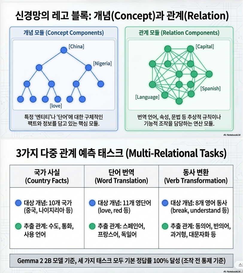
같은 semantic concept를 표현하는 feature들은 여러 layer에서 동시에(coactivate) 활성화될 것이다.

예를 들어,

"What is the capital of China?"

에서는 China feature, Capital feature, Answer feature(Beijing)들이 동시에 활성화된다.

이들을 network로 연결하면 China module, Capital module을 얻을 수 있다는 것이다.

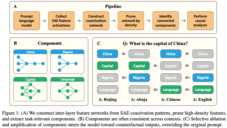
전체 Pipeline

논문의 pipeline은 매우 간단하다.

Prompt
↓
Run LLM + SAE
↓
Collect sparse feature activations
↓
Build coactivation graph
↓
Prune graph
↓
Connected Components
↓
Causal Intervention

Figure 1이 바로 이 전체 과정을 보여준다.

2. 방법론

Step1. SAE activation 추출

모든 residual layer에 대해 SAE encoder를 적용한다.

원래 residual: $x_\ell$

SAE feature: $\phi_\ell=Encoder(x_\ell)$

feature dimension: 16384 이다.

토큰별 activation은 $\Phi_\ell\in R^{T\times16384}$ 가 된다.

여기서 T는 token 개수이다.

Step2. 중요한 feature 선택

모든 feature를 쓰면 너무 많다.

그래서 각 token마다 Top-5 activation만 선택한다.

수식은 $S_\ell=\bigcup_t\text{TopK}(\Phi_\ell[t])$

즉, layer마다 Top5 feature만 남긴다.

Step3. Coactivation Graph 구축

논문의 핵심이다.

Node: (layer, feature) 이다.

예:

Layer10, feature125
↓
Layer11, feature430

Edge는 Pearson correlation으로 연결한다.

$\rho=corr(\Phi_\ell[:,i],\Phi_{\ell+1}[:,j])$

만약 $\rho>0.9$ 이면 edge 생성.

즉, feature A와 feature B가 prompt 전체 token에 대해 비슷하게 activation하면 연결한다.

Step4. Graph Pruning

문제는 자주 켜지는 feature이다.

예:

space, period, common syntax 이런 feature는 모든 prompt에서 켜진다.

논문은 Neuronpedia activation density를 이용한다.

activation density $d_i$ 가 0.01 이하만 남긴다.

즉, 희귀한 sparse feature만 유지한다.

Step5. Connected Component 추출

이제 graph는 node들이 연결되어 있다.

NetworkX의 BFS로 Connected Component를 찾는다.

예:

China
↓
country
↓
Asia
↓
Beijing

이 하나의 module이 된다.

Step6. Causal Validation

단순히 graph를 찾는 것으로 끝나지 않는다.

논문은 실제로 해당 component를 ablation한다.

즉, component 내 feature activation을 0으로 만든다.

그리고 출력 분포 변화를 측정한다.

평가는 KL divergence $KL(P_{original},P_{ablated})$ 이다.

KL이 크면 해당 component가 실제로 중요한 것이다.

Steering

논문의 가장 재미있는 부분이다.

예를 들어,

Prompt: Capital of China?

원래 China component, Capital component가 활성화된다.

이제 China component를 끄고 Nigeria component를 증폭한다.

그러면 Abuja가 나온다.

즉,

China
↓
Nigeria

로 semantic module을 교체한 것이다.

Composite Steering

더 재미있는 것은 동시에

China --> Nigeria, Capital --> Language를 바꾸는 것이다.

그러면 “Capital of China?”가 English로 바뀐다.

즉, Concept와 Relation module이 독립적으로 합성(composition) 가능하다는 것을 보여준다.

3. 실험

논문은 3개의 task를 사용한다.

(1) Country Facts

Concept:

China
Nigeria
...

Relation:

Capital
Currency
Language

(2) Translation

Concept:

love
red
...

Relation:

Spanish
French
German

(3) Verb Transformation

Concept:

break
hide
...

Relation:

past tense
capitalization
synonym

Gemma-2B는 세 작업 모두에서 원래 정확도 100%를 보였다.

실험 1. 중요한 Component 찾기

Figure 2의 결과에서 Component마다 feature 수와 KL divergence를 그려 보면

대부분의 component는 KL≈0 이다.

하지만 2~3개의 component만 KL이 매우 크다.

즉, 실제로 causal한 module은 극히 일부라는 것이다.

실험 2. Context Consistency

논문의 매우 중요한 발견이다.

예를 들어,

China component를

Capital, Currency, Language에서 각각 추출하면

거의 동일한 graph가 나온다.

즉, China module은 relation과 무관하게 항상 동일하다.

이것이 semantic module이라고 주장한다.

실험 3. Steering 성능

Table 2의 평균 성공률은 다음과 같다.

Steering 종류	평균 성공률
Concept steering	96% (Country Facts), 75% (Translation), 48% (Verb)
Relation steering	93%, 98%, 23%
Concept+Relation steering	90%, 64%, 19%

주요 해석은 다음과 같다.

Country Facts에서는 개념과 관계가 매우 독립적으로 구성되어 있어 steering이 거의 완벽하게 동작한다.
Translation도 높은 성공률을 보이며, 언어(language)와 단어(word)가 상당히 분리된 표현을 가진다.
Verb Transformation은 synonym, antonym, past tense처럼 문맥 의존성이 강한 관계이므로 성공률이 크게 떨어진다.

실험 4. Layer 분석

Figure 4에서 매우 흥미로운 결과가 나온다.

Concept

대부분 Layer0부터 등장한다.

예: China, Nigeria, love

Relation

대부분 후반 layer에서 등장한다.

예: Capital, Language, Currency

즉,

Early Layer
Entity
↓
Late Layer
Relation

이라는 계층적 구조를 보여준다. 이는 LLM이 먼저 구체적 개체를 표현하고, 이후 관계를 조합한다는 해석과 일치한다.

실험 5. Single Feature vs Component

기존 SAE 연구는 feature 하나만 steering한다.

논문은 비교 실험을 수행했다.

Country Facts 평균

방법	성공률
Single Feature	83% / 83% / 75%
Component	96% / 93% / 90%

즉, Component가 훨씬 강력하다.

이는 semantic information이 하나의 feature가 아니라 feature group에 분산되어 있다는 증거라고 주장한다.

실험 6. Specificity

다른 task에 영향이 있는지도 평가했다.

예를 들어,

Country component를 ablation해도 Verb task 정확도는 100% 유지된다.

반면 Verb component는 다른 task에도 영향을 준다.

이는 Country component가 상당히 task-specific이라는 의미이다.

논문의 기여

SAE feature를 개별 단위가 아닌 module(connected component) 단위로 해석했다.
복잡한 EAP나 Activation Patching 없이, feature coactivation만으로 의미 있는 semantic module을 추출했다.
Concept와 Relation이 독립적으로 조합 가능함을 인과적 개입(steering)으로 검증했다.
Entity는 초기 layer, Relation은 후기 layer에 집중된다는 계층적 구조를 제시했다.

** Sparse Feature Coactivation Reveals Causal Semantic Modules in Large Language Models (ArXiv 2025)

1. 연구 배경

(1) Circuit Discovery

(2) SAE Feature

핵심 아이디어

전체 Pipeline

2. 방법론

Step1. SAE activation 추출

Step2. 중요한 feature 선택

Step3. Coactivation Graph 구축

Step4. Graph Pruning

Step5. Connected Component 추출

Step6. Causal Validation

Steering

Composite Steering

3. 실험

(1) Country Facts

(2) Translation

(3) Verb Transformation

실험 1. 중요한 Component 찾기

실험 2. Context Consistency

실험 3. Steering 성능

실험 4. Layer 분석

Concept

Relation

실험 5. Single Feature vs Component

실험 6. Specificity

논문의 기여

댓글

답글 남기기 응답 취소