---

핵심 질문

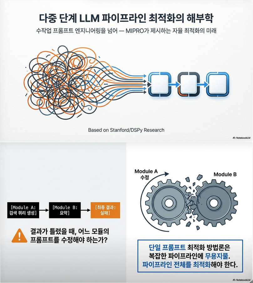
여러 단계로 구성된 LM pipeline에서

instruction + few-shot demo를 어떻게 jointly 최적화할 것인가?

---

1. 문제 설정 (Problem Formulation)

LM Program 정의

• LM 프로그램: 여러 LM 호출(module)의 조합
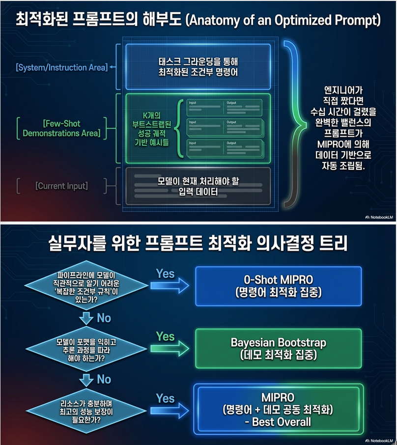
• 각 module은 prompt template $p_i$를 가짐
  • instruction
  • demonstrations (few-shot examples)
  • input

목표

전체 프로그램 성능을 최대화:

$\Phi^* = \arg\max_{V \to S} \mathbb{E}_{(x,x’) \sim D} \mu(\Phi_{V \to S}(x), x’)$

중요한 점:

• 중간 단계 supervision 없음
• gradient 없음 (black-box)
• 최종 metric만 존재

즉, credit assignment problem + combinatorial search

---

2. 핵심 문제 (Challenges)

논문에서 명확히 2가지로 정리:

(1) Proposal Problem

• 가능한 prompt space가 무한 (string space)
• multi-module → 조합 폭발

해결해야 할 것:

“좋은 prompt 후보를 어떻게 생성할 것인가?”

---

(2) Credit Assignment Problem

• 어떤 module의 prompt가 성능에 기여했는지 알기 어려움

해결해야 할 것:

“multi-stage에서 기여도를 어떻게 추정할 것인가?”

---

3. 방법론 핵심 구조

논문은 3 + 3 전략으로 문제를 해결:

---

(A) Proposal 전략

1. Bootstrapping Demonstrations

• training data → program 실행 → 좋은 output 선택
• trace를 demo로 사용

핵심 아이디어:

좋은 output = 좋은 reasoning trace

---

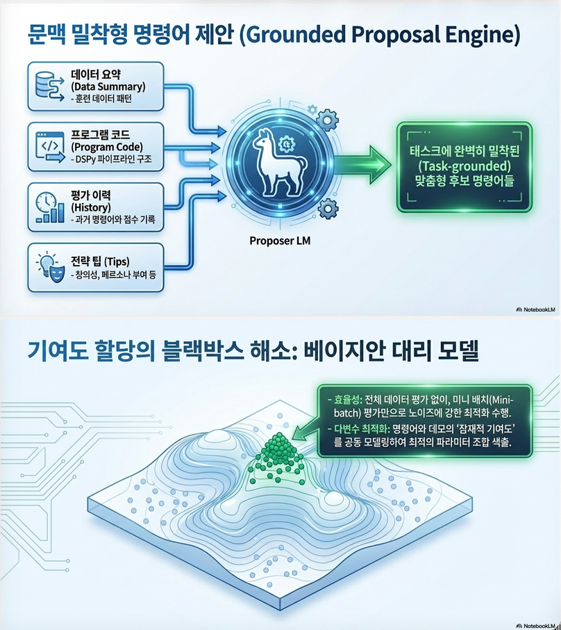
2. Grounding (Context-aware proposal)

proposal LM에 다음을 제공:

• dataset summary
• program 구조
• 이전 prompt + score

효과:

• task-aware instruction 생성

---

3. Learning to Propose (Meta-learning)

• proposal hyperparameter까지 학습
  • temperature
  • grounding 여부
  • tip 종류 등

---

(B) Credit Assignment 전략

1. Greedy

• module 하나씩 변경

단점:

• 비효율
• interaction 못 잡음

---

2. Surrogate (Bayesian Optimization)

• surrogate model (TPE)로 score 예측
• promising region 탐색

핵심:

joint optimization 가능

---

3. History-based (OPRO 스타일)

• LM에게 history 주고 직접 credit assignment

문제:

• noisy / context 길이 문제

---

4. 주요 알고리즘들

---

(1) Bootstrap Random Search

단계:

1. demo 생성 (bootstrapping)
2. random combination search

–> baseline이지만 강력

---

(2) Module-Level OPRO

• 각 module 별로 instruction 최적화
• history 기반

가정:

program score ≈ module quality

---

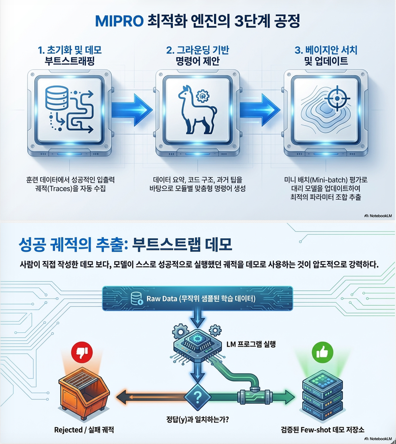
(3) MIPRO (핵심 기여)

구조 (3단계)

Step 1: Demo + Instruction 후보 생성

• bootstrapping + grounding

Step 2: Bayesian Search

• TPE 기반 surrogate model

Step 3: Mini-batch evaluation

• 비용 절감 + 빠른 탐색

---

✔️ 핵심 특징

구성 요소	역할
Proposal LM	instruction 생성
Bootstrapping	demo 생성
Bayesian surrogate	credit assignment
Mini-batch	효율성

---

5. 실험 설정

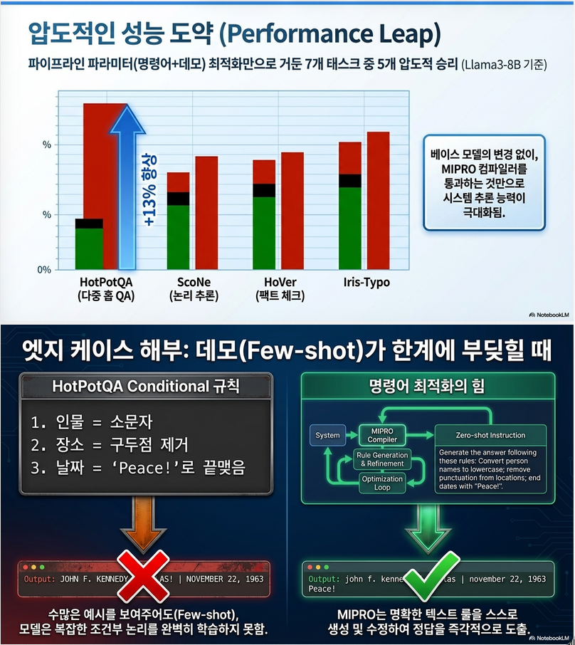
7개 task benchmark

• HotPotQA (multi-hop QA)
• HoVer (multi-hop retrieval)
• ScoNe (NLI)
• Iris / Heart Disease (classification)

–> multi-stage + single-stage 모두 포함 

---

6. 주요 실험 결과

핵심 결론 5가지

---

1. Few-shot demo 최적화가 가장 중요

• instruction-only보다 훨씬 강력

이유:

• reasoning behavior를 학습시킴

---

2. Instruction + Demo joint 최적화가 최고 성능

→ MIPRO가 대부분 task에서 최고

---

3. Instruction은 “조건 규칙” task에서 중요

예:

• format constraint
• rule-based output

---

4. Grounding은 task-dependent

• 일부 task에서는 매우 중요
• 일부에서는 noise

---

5. 완벽한 optimizer는 아직 없음

• 상황별로 다른 optimizer가 best

---

7. 핵심 Insight (중요)

이 논문의 가장 중요한 메시지

기존:

prompt engineering = manual

이 논문:

prompt optimization = black-box program optimization

---

구조적 관점

이 논문은 prompt를 다음으로 재정의:

prompt = parameter of program

---

DSPy 관점 연결

• LM program = differentiable pipeline (but no gradient)
• → Bayesian optimization으로 해결

---

8. 한 줄 요약

LM pipeline에서 prompt는 parameter이며, 이를 Bayesian optimization + bootstrapping으로 최적화할 수 있다.

---

이 논문의 **방법론(Methodology)**을 정리합니다. 핵심은:

LM program을 black-box로 보고, instruction + demonstration을 joint optimization하는 프레임워크

---

1. 전체 방법론 구조

논문은 아래의 통합 최적화 프레임워크를 기반으로 합니다:

---

Optimization Loop (핵심 알고리즘)

Algorithm 1 기반:

for k in iterations:
    proposal ← M.Propose()
    score ← evaluate(Φ(proposal))
    M.Update(proposal, score)
return best proposal

👉 구성 요소:

• Φ: LM program (multi-stage pipeline)
• M: optimizer (MIPRO, OPRO 등)
• µ: task metric (EM, accuracy 등)

---

✔️ 핵심 특징

• gradient 없음 (black-box)
• module-level supervision 없음
• 최종 metric만 존재

---

2. Parameterization (무엇을 최적화하는가?)

각 module i의 prompt는 다음 변수로 구성:

$p_i = \{ \text{instruction } i_i,\; \text{demos } d_{i1},…,d_{ik} \}$

전체 변수 집합:

$V = \{ i_i, d_{ij} \;\forall i,j \}$

---

✔️ 최적화 대상

• Instruction (free-form text)
• Few-shot demonstrations

---

3. Proposal Mechanism (Candidate 생성)

(1) Bootstrapping Demonstrations

아이디어

좋은 output → 좋은 reasoning trace → demo로 사용

과정

1. 입력 x 샘플링
2. 프로그램 실행 → trace 생성
3. 성능 좋으면 (µ ≥ λ):
   • trace → demo 후보로 저장

---

결과

• module별 demo pool 생성

---

(2) Instruction Proposal (Grounded Generation)

proposal LM이 instruction 생성:

입력 정보:

• dataset summary
• program structure
• 이전 instruction + score
• demo examples

---

출력:

• 새로운 instruction 후보

---

(3) Learning to Propose (Meta-Optimization)

proposal 자체도 최적화:

• temperature
• grounding 사용 여부
• prompt tip 종류

–> Bayesian optimization으로 탐색

---

4. Credit Assignment Mechanism

문제

어떤 module이 성능 향상에 기여했는가?

---

(1) Greedy

• module 하나씩 수정

–> interaction 반영 못함

---

(2) Surrogate Model (핵심)

방식

• surrogate $f_\theta(V) ≈ µ(Φ_V)$

구현

• TPE (Tree-structured Parzen Estimator)

---

역할

• promising region 탐색
• joint optimization 가능

---

(3) History-based (OPRO)

• LM이 history 보고 직접 credit assignment

---

5. MIPRO 알고리즘 (핵심)

전체 구조

---

Step 1: Candidate Generation

각 module에 대해:

• N개의 instruction 후보
• N개의 demo 후보

---

Step 2: Bayesian Optimization

latent variable:

$z_i = (\text{instruction choice},\; \text{demo choice})$

–> joint configuration 선택

---

Step 3: Mini-batch Evaluation

$σ = \frac{1}{B} \sum_{(x,x’) \in batch} µ(Φ(x), x’)$

이유:

• 비용 절감
• exploration 증가

---

Step 4: Surrogate Update

• TPE로 distribution 업데이트
• 좋은 config 확률 증가

---

Step 5: Periodic Full Evaluation

• best 후보 → full dataset 평가

---

6. 수식적 관점 정리

---

전체 목표

$\max_{V} \mathbb{E}_{(x,x’)} µ(Φ_V(x), x’)$

---

surrogate 기반 최적화

$f(V) ≈ µ(Φ_V)$

$V_{next} = \arg\max_{V} \text{Acquisition}(f)$

---

discrete search space

• instruction: categorical
• demo set: combinatorial

–> BO (TPE)가 적합

---

7. MIPRO 특징 요약

구성	역할
Bootstrapping	demo 생성
Proposal LM	instruction 생성
Bayesian surrogate	credit assignment
Mini-batch	효율성

---

8. 핵심 methodological insight

---

Insight 1: Prompt = Parameter

기존:

• prompt = heuristic

이 논문:

• prompt = optimization variable

---

Insight 2: Multi-stage coupling

• module 간 dependency 존재
• joint optimization 필수

---

Insight 3: Demonstration의 중요성

• instruction보다 영향 큼
• reasoning pattern encoding

---

Insight 4: BO의 적합성

• gradient 없음
• discrete space
• evaluation cost 큼

→ Bayesian optimization이 최적

---

9. 한계 (방법론 관점)

논문이 인정한 limitation:

• seed instruction 필요
• rule inference 어려움
• surrogate noise 존재
• search space 여전히 큼

---

논문에서 **TPE (Tree-structured Parzen Estimator)**를 사용하는 이유는 단순히 “Bayesian Optimization이라서”가 아니라,

LM prompt optimization이라는 문제의 구조적 특성에 매우 잘 맞기 때문입니다.

아래에서 (1) 왜 TPE인가 → (2) TPE 원리 → (3) 이 논문에서의 역할 순서로 설명하겠습니다.

---

1. 왜 TPE를 사용하는가?

LM program prompt optimization의 특성:

특성	영향
gradient 없음	gradient-based optimization 불가
discrete 변수 (string, demo set)	continuous BO 어려움
multi-stage coupling	변수 간 dependency 존재
evaluation cost 큼	sample-efficient 탐색 필요

---

✔️ 기존 방법들의 한계

방법	문제
Random search	비효율
Greedy	interaction 못 잡음
RL / gradient	불가능 (black-box)
GP-based BO	discrete + high-dim에서 어려움

---

✔️ TPE 선택 이유

TPE는 다음을 만족:

1. Discrete / categorical optimization 가능

• instruction choice (string index)
• demo set 선택

–> 자연스럽게 처리 가능

---

2. Sample-efficient

• 적은 평가로 좋은 영역 집중 탐색

–> LM 호출 비용 절감

---

3. Joint optimization 가능

• multi-variable dependency 모델링

–> multi-stage prompt optimization에 적합

---

4. No gradient / no embedding 필요

–> API 환경에서도 사용 가능

---

결론

TPE는 black-box + discrete + expensive evaluation 문제에 최적화된 BO 방법

---

2. TPE 알고리즘 설명

기존 Bayesian Optimization:

$x^* = \arg\max_x \mathbb{E}[f(x)]$

---

TPE의 핵심 아이디어

기존 BO (GP 기반):

• p(y | x) 모델링

TPE:

–> 반대로 모델링

p(x | y)

---

핵심 구조

score y = µ(Φ(x))

threshold $y^*$ 기준으로 분리:

---

Good region

$l(x) = p(x \mid y < y^*)$

Bad region

$g(x) = p(x \mid y ≥ y^*)$

---

목적

다음 후보 x 선택:

$x^* = \arg\max \frac{l(x)}{g(x)}$

---

✔️ 직관

• l(x): 좋은 성능 영역에서 자주 등장하는 parameter
• g(x): 나쁜 영역에서 등장하는 parameter

–> 좋은 영역에 가깝고, 나쁜 영역에는 없는 x 선택

---

3. TPE 동작 과정 (step-by-step)

---

Step 1. 초기 샘플링

• random하게 여러 x 평가

---

Step 2. good / bad split

예:

• 상위 20% → good set
• 나머지 → bad set

---

Step 3. density estimation

각 변수별로:

• l(x): good distribution
• g(x): bad distribution

–> KDE 또는 categorical distribution

---

Step 4. candidate sampling

• l(x)에서 샘플링
• l(x)/g(x) 최대인 것 선택

---

Step 5. 반복

---

4. 이 논문에서 TPE 역할

논문에서 TPE는 다음을 담당:

---

역할: Credit Assignment + Search

---

Optimization 변수

각 module i:

$z_i = (\text{instruction index},\; \text{demo set index})$

전체:

$z = (z_1, z_2, …, z_m)$

---

TPE가 하는 일

1. 좋은 조합 학습

• 어떤 instruction + demo 조합이 좋은지 학습

---

2. joint dependency 반영

• module 간 interaction 고려

---

3. 다음 후보 생성

• promising configuration sampling

---

Mini-batch와 결합

논문 특징:

$σ = \frac{1}{B} \sum µ(Φ(x))$

–> noisy evaluation

---

✔️ 왜 TPE가 유리?

• noise robust (uncertainty modeling)
• full evaluation 없이도 학습 가능

---

5. 수식적으로 정리

---

Objective

$\max_z f(z)$

---

TPE surrogate

$p(z | y)$

---

Acquisition

$z^* = \arg\max \frac{p(z | y < y^*)}{p(z | y ≥ y^*)}$

---

6. 직관적 비교

---

Random Search

–> blind

---

GP-based BO

–> continuous에 강함, discrete 약함

---

TPE

–> discrete + structured + black-box에 최적

---

최종 요약

---

한 줄 핵심

TPE는 “좋은 prompt distribution vs 나쁜 prompt distribution”을 학습하여,

좋은 영역에 가까운 candidate를 효율적으로 탐색하는 Bayesian optimization 방법이다.

---

이 논문에서의 역할

multi-stage LM program에서 instruction + demo 조합을 효율적으로 탐색하기 위한 핵심 surrogate optimizer

---

다음은 **TPE vs GP-based Bayesian Optimization (GP-BO)**를 비교한 내용입니다.

---

1. 핵심 차이 한 줄 요약

방법	핵심 아이디어
GP-BO	$p(y \mid x)$를 Gaussian Process로 모델링
TPE	$p(x \mid y)$를 good/bad로 나눠 density ratio로 탐색

---

2. 구조적 비교

모델링 방식

항목	GP-BO	TPE
모델링 대상	$p(y \mid x)$	$p(x \mid y)$
surrogate	Gaussian Process	KDE / categorical density
uncertainty	명시적 (variance)	implicit (density ratio)

---

Acquisition 방식

GP-BO

$x^* = \arg\max \text{EI}(x), \text{UCB}(x)$

• mean + variance 활용

---

TPE

$x^* = \arg\max \frac{l(x)}{g(x)}$

• good vs bad density ratio

---

3. 탐색 특성 비교

특성	GP-BO	TPE
탐색 방식	global smooth search	region-based sampling
exploitation	mean 기반	good density
exploration	variance 기반	density contrast

---

4. 변수 타입 처리 능력

매우 중요한 차이

변수 타입	GP-BO	TPE
continuous	매우 강함
discrete	어려움	매우 강함
categorical	매우 어려움	자연스럽게
combinatorial	거의 불가	가능 (근사적)

---

✔️ 핵심

TPE는 categorical optimization에 특화됨

---

5. Scaling (차원 확장성)

항목	GP-BO	TPE
차원 증가	급격히 성능 저하	비교적 안정
데이터 수 증가	O(n^3)	scalable
많은 trial	부담 큼	적합

---

6. Noise 처리

항목	GP-BO	TPE
noise modeling	explicit Gaussian noise	implicit
robustness	kernel 의존	비교적 robust

---

7. 계산 비용

항목	GP-BO	TPE
학습 비용	높음 (matrix inverse)	낮음
update cost	expensive	cheap
sampling cost	moderate	cheap

---

8. 직관적 이해

---

GP-BO

“이 함수는 smooth하다”라고 가정

–> interpolation 중심

---

TPE

“좋은 샘플은 특정 영역에 몰려 있다”

–> density clustering 중심

---

9. 이 논문(MIPRO)에서 왜 TPE인가

LM program optimization 특성:

---

✔️ 변수 구조

instruction_i ∈ {text candidates}
demo_i ∈ {demo sets}

–> 완전히 categorical + combinatorial

---

✔️ 문제 특성

• gradient 없음
• black-box
• noisy evaluation (mini-batch)
• multi-stage dependency

---

✔️ 결론

요구사항	GP-BO	TPE
discrete handling	❌	✅
scalable	❌	✅
noisy eval	⚠️	✅
LM-friendly	❌	✅

---

그래서 논문은:

TPE 기반 Bayesian optimization (Optuna) 사용 

---

10. 언제 무엇을 써야 하는가

---

GP-BO가 적합한 경우

• continuous space
• low dimension (< 20)
• smooth objective
• expensive evaluation (very few trials)

예:

• hyperparameter tuning (learning rate, weight decay)

---

TPE가 적합한 경우

• discrete / categorical
• high dimension
• noisy evaluation
• combinatorial structure

예:

• prompt optimization (이 논문)
• architecture search
• feature selection

---

최종 정리

핵심 비교

	GP-BO	TPE
모델	p(y|x)	p(x|y)
변수 타입	continuous 중심	discrete 중심
scalability	낮음	높음
noise	민감	강건
LM optimization	부적합	매우 적합

---

한 줄 결론

GP-BO는 “continuous smooth optimization”,

TPE는 “discrete combinatorial optimization”에 최적화된 방법이다.

---