---

1. 문제의식: LLM 기반 “탐색”의 한계

최근 LLM을 테스트 타임에서 여러 번 샘플링하여 더 나은 해를 찾는 방식(test-time compute scaling)이 주목받고 있습니다.

하지만 기존 방식들은 다음 한계를 가집니다:

접근	한계
Repeated Sampling	탐색 공간 구조를 고려하지 않음
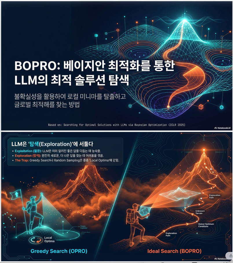
Greedy OPRO	exploitation 위주 → local optima에 갇힘
진화 알고리즘	비용 큼 / 정적 전략
난이도 예측 기반 전략 선택	실전에서 task difficulty 예측 어려움

핵심 질문

LLM 기반 탐색에서 exploration–exploitation trade-off를 자동으로 조절할 수 있는가?

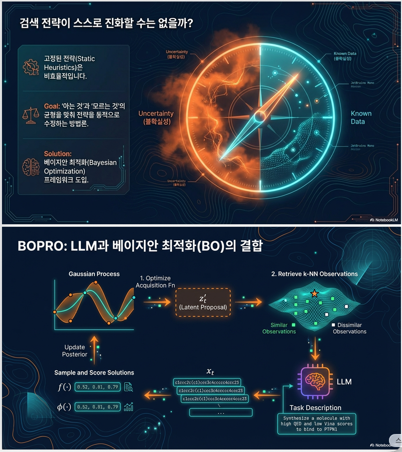
이 논문은 여기에 대해 **Bayesian Optimization(BO)**을 활용한 해법을 제안합니다.

---

2. 제안 방법: Bayesian-OPRO (BOPRO)

핵심 아이디어

LLM을 단순히 반복 샘플링하지 않고,

1. 잠재 공간(latent embedding space)에서 BO 수행
2. BO가 제안한 latent vector 주변을 LLM이 생성하도록 프롬프트 구성

즉,

$\text{LLM search} + \text{Bayesian surrogate uncertainty}$

---

전체 구조 (Figure 1, p.2)

반복 루프 (iteration t)

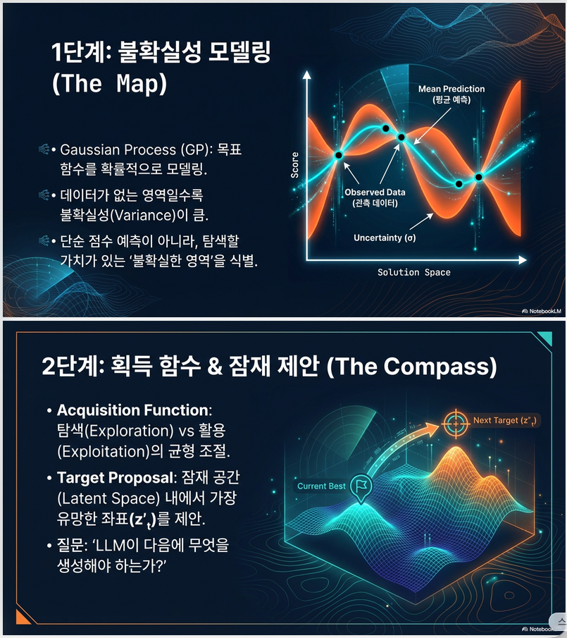
① Surrogate 모델 (GP)

이전 해들 $(z_i, f(x_i))$로부터

$p(f(x) | \mathcal{D}_{1:t-1})$

를 추정

---

② Acquisition 최적화

$z’_t = \arg\max_z \alpha(z)$

• LogEI
• UCB
• Thompson Sampling

→ 다음에 탐색할 “유망한 잠재 위치” 결정

---

③ Latent → Text 디코딩

BO가 제안한 $z’_t$와 cosine similarity가 높은 이전 해 k개를 골라

→ 이를 in-context example로 사용

→ LLM이 새로운 해 $x_t$ 생성

---

④ 평가 및 업데이트

$z_t = \phi(x_t)$

black-box score 계산 → GP posterior 업데이트

---

이 과정을 반복

---

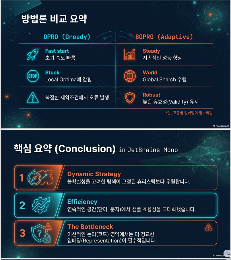
3. OPRO와의 차이

기존 OPRO:

• top-k (score 기준) 해를 prompt에 넣음
• 완전 greedy
• exploitation 중심

BOPRO:

• latent similarity 기준 선택
• GP uncertainty 활용
• exploration/exploitation 자동 균형

예시 (Semantle):

기존 단어	score
word	0.7
sentence	0.65
lock	0.5
metal	0.49

OPRO → word, sentence

BOPRO → lock, metal 선택 가능 → locksmith → wordsmith

---

4. 실험 설정

3개 탐색 문제에 적용:

---

(1) Semantle (단어 찾기)

• hidden word 찾기
• similarity 점수만 피드백
• 최대 1000 guess

---

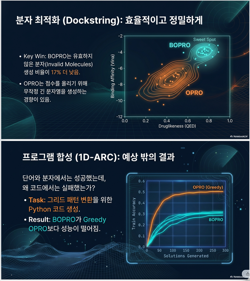
(2) Dockstring (분자 최적화)

목표:

• QED (drug-likeness)
• Vina (binding affinity)

scalarized objective:

$0.2 \cdot QED + 0.8 \cdot NNV$

결과는 Figure 2(b), p.7

---

(3) 1D-ARC (가설 + 프로그램 탐색)

• 자연어 알고리즘 + Python 코드 생성
• train grid 모두 맞추는 프로그램 탐색

---

5. 주요 결과

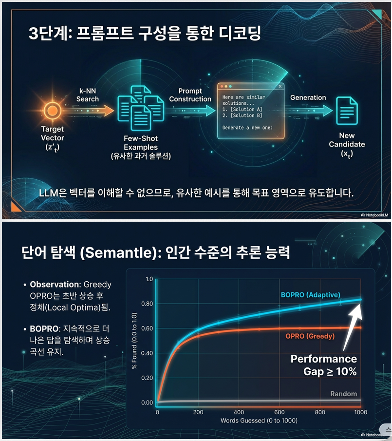
Semantle (Figure 2a)

• BOPRO가 OPRO보다 ≥10%p 높음
• OPRO는 초반 급상승 후 plateau
• BOPRO는 steady improvement

→ local optimum 탈출 가능

---

Dockstring (Figure 2b)

• BOPRO가 약간 더 높은 최적값
• OPRO는 17% 더 많은 invalid molecule 생성
• OPRO는 58개 중 12개 target만 완료

→ greedy는 분자 길이 과도 증가

---

1D-ARC (Figure 2c)

• BOPRO가 OPRO보다 낮음
• 심지어 RS보다도 낮음

---

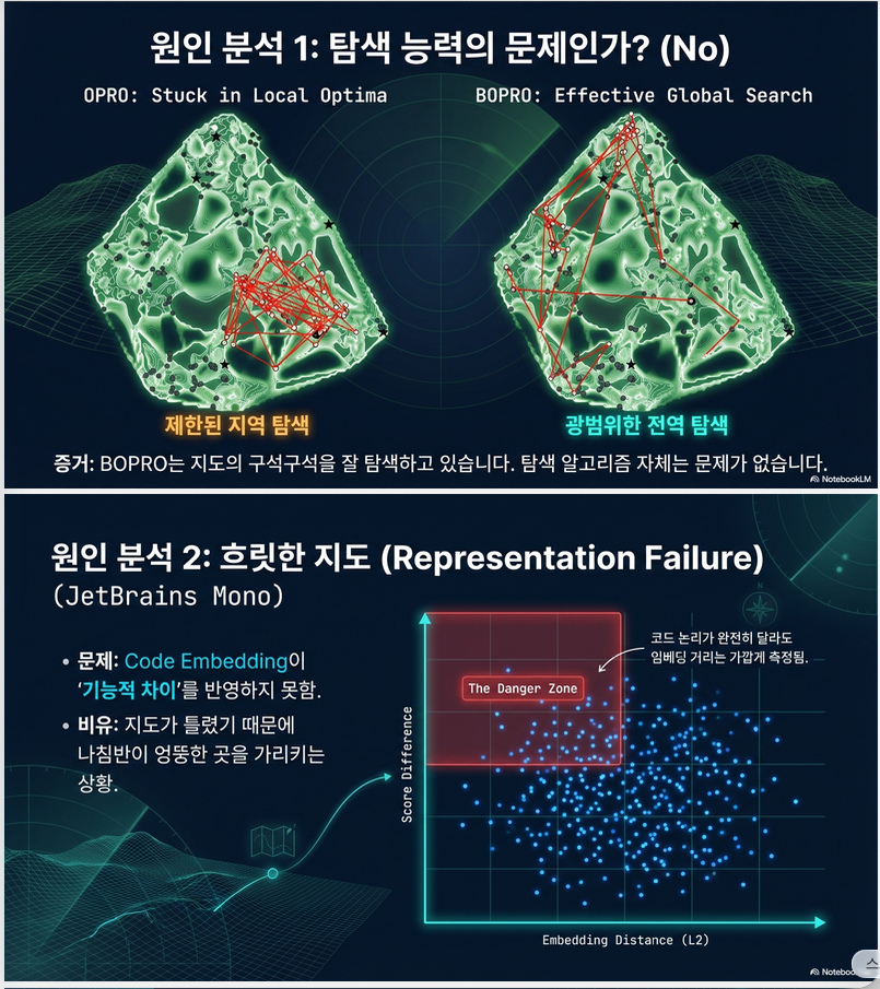
6. 실패 원인 분석 (Section 8)

질문 1: BOPRO가 exploration 못했나?

아님.

Figure 5 (p.9):

• low warm-start 문제에서 BOPRO는 잘 탐색함
• bimodal distribution → exploration/exploitation 균형

---

질문 2: Representation 문제?

Figure 6 (p.10)

scatter plot:

• x축: embedding distance
• y축: score difference

문제:

• L2 distance 작아도 score 차이 큼

즉,

코드 embedding이 fine-grained semantic 차이를 못 잡음

예:

if x > 3:

vs

if x >= 3:

embedding은 거의 동일

하지만 결과는 완전히 다름

→ GP surrogate가 의미 있는 smooth function을 학습 불가

---

7. 결론

Task	결과
Word search	BOPRO 우수
Molecule opt	BOPRO 우수
Program search	representation 한계로 실패

---

8. 이 논문의 이론적 의미

(1) LLM search = BO 문제로 재해석

LLM generation을 black-box optimization으로 공식화

---

(2) In-context optimization의 Bayesian generalization

OPRO → greedy heuristic

BOPRO → uncertainty-aware search

---

(3) Representation quality가 BO 성능의 병목

이 논문이 암묵적으로 말하는 것:

“LLM + BO”의 성패는 embedding geometry에 달려있다

---

다음은 논문의 **방법론(Methodology)**을 수식과 알고리즘 관점에서 정리한 것입니다 

---

1. 문제 정식화

우리는 다음 black-box 최적화 문제를 푼다:

$x^* = \arg\max_{x \in \mathcal{A}} f(x)$

• x: LLM이 생성하는 텍스트 해 (단어, SMILES, 코드 등)
• f(x): 외부 검증기(black-box score)
• $\mathcal{A}$: 가능한 해 공간
• 예산 T: 평가 가능 횟수 제한

문제점:

텍스트 공간은 이산 + 고차원 → 직접 BO 불가능

---

2. 핵심 아이디어

Latent-space Bayesian Optimization

1. 텍스트 해를 embedding으로 매핑 $z = \phi(x) \in \mathbb{R}^d$
2. latent 공간에서 BO 수행
3. BO가 제안한 latent 위치 주변을 LLM이 생성하도록 프롬프트 구성

즉,

$\text{Text Optimization} \rightarrow \text{Embedding-space BO}$

---

3. 전체 알고리즘 구조 (BOPRO)

반복 루프 (iteration t)

---

3.1 Warm Start

LLM으로 W개의 초기 해 생성

$\{(x_w^{(i)}, f(x_w^{(i)}))\}_{i=1}^W$

embedding 계산:

$z_w^{(i)} = \psi(\phi(x_w^{(i)}))$

• $\phi$: embedding model
• $\psi$: optional dimensionality reduction (보통 identity)

---

3.2 Surrogate 모델 (Gaussian Process)

Latent space에서 GP 구성:

$f(z) \sim \mathcal{GP}(m(z), k(z,z’))$

• kernel: Matern 5/2
• posterior:

$p(f(z) | \mathcal{D}_{1:t-1}) = \mathcal{N}(\mu_t(z), \sigma_t^2(z))$

---

3.3 Acquisition Function 최적화

다음 탐색 지점:

$z’_t = \arg\max_z \alpha(z)$

사용한 acquisition:

(1) Log Expected Improvement

$EI(z) = \mathbb{E}[\max(f(z) – f^+, 0)]$

(2) Upper Confidence Bound

$UCB(z) = \mu_t(z) + \beta \sigma_t(z)$

(3) Thompson Sampling

$f^{(s)} \sim \text{posterior}, \quad z’_t = \arg\max f^{(s)}(z)$

---

4. Latent → Text 디코딩 (핵심 부분)

BO는 continuous latent vector $z’_t$를 제안

하지만 우리는 텍스트를 생성해야 함

---

4.1 Similarity 기반 In-context Prompt 구성

이전 해들:

$Z = \{z_w^{(i)}\} \cup \{z_j\}_{j=1}^{t-1}$

각 해와 cosine similarity 계산:

$s(z’_t, z_i)$

상위 k개 선택 → prompt 구성

---

4.2 LLM Generation

프롬프트에 k개 해 포함 후

$x_t \sim p_\theta(x | \text{prompt}(z’_t))$

batch decoding 사용

---

4.3 평가 및 업데이트

$f(x_t)$

$z_t = \psi(\phi(x_t))$

데이터셋 업데이트:

$\mathcal{D}_t = \mathcal{D}_{t-1} \cup \{(z_t, f(x_t))\}$

GP posterior 업데이트

---

5. OPRO와의 차이

OPRO	BOPRO
score 기반 top-k	latent similarity 기반
greedy exploitation	uncertainty-aware
local optima 위험	exploration 가능

BOPRO는 OPRO의 Bayesian generalization

---

6. Error Handling

중복 생성

• 재샘플링
• 실패 시 BO proposal을 surrogate 업데이트에 사용

Invalid output

• self-refine loop
• 실패 시 score = -1

---

7. 알고리즘 요약 (Pseudo-code)

Initialize warm-start set
Compute embeddings

for t = 1 to T:
    Fit GP on (z_i, f_i)

    z_t' = argmax acquisition(z)

    Select k past solutions most similar to z_t'
    Construct prompt

    x_t = LLM(prompt)
    score = f(x_t)

    z_t = embedding(x_t)
    Add (z_t, score) to dataset

Return best x

---

8. 방법론의 핵심 기여

(1) LLM 탐색을 BO 문제로 정식화

(2) Latent-space surrogate 구축

(3) In-context prompting을 acquisition-driven sampling으로 재해석

---

9. 방법론의 이론적 장점

• Adaptive exploration
• Task difficulty에 자동 적응
• 정적 heuristic 불필요
• Greedy 대비 global optimum 탐색 가능성 증가

---

10. 병목 지점

핵심 가정:

$\text{Embedding distance} \approx \text{Score smoothness}$

1D-ARC에서 실패 원인:

• 코드 embedding이 fine-grained semantic 차이 반영 못함
• GP가 smooth function 학습 불가

즉,

Representation quality가 BO 성능을 결정

---

embedding model, dimensionality reduction 모델 구성(학습을 따로 하는가?), kernel: Matern 5/2 설명, Latent → Text 디코딩 예를 들어 설명

---

1. Embedding Model 구성

어떤 모델을 사용했는가?

Task별로 off-the-shelf embedding 모델을 사용합니다.

Task	Embedding 모델
Semantle	GTE-Qwen-2-1.5B-Instruct
1D-ARC	GTE-Qwen-2-1.5B-Instruct (code + text 학습됨)
Dockstring	Molformer (SMILES 특화)

---

학습을 따로 하는가?

아니오.

• embedding model은 사전학습(pretrained) 모델을 그대로 사용
• BO 과정 중 embedding을 업데이트하지 않음
• representation learning은 수행하지 않음

즉,

$z = \phi(x)$

는 고정 함수입니다.

---

왜 fine-tuning을 하지 않았는가?

논문 목표는:

“LLM search 전략을 개선하는 것”

representation learning은 범위 밖으로 둠.

그러나 1D-ARC 실패 분석에서:

코드 embedding 품질이 문제

라고 명확히 지적합니다 (Section 8.2).

---

2. Dimensionality Reduction 모델 구성

논문에서 언급된 ψ(·):

$z = \psi(\phi(x))$

가능한 옵션:

• PCA
• Random Projection
• Low-rank projection

---

학습 여부?

PCA:

• warm-start 또는 unlabeled set 기반으로 fitting 가능
• 그러나 논문 기본 설정은:

dimensionality reduction을 사용하지 않는 것이 가장 성능이 좋음

즉,

$\psi = I$

(Identity)

---

왜 reduction이 필요할 수 있는가?

GP는 high-dim에서 어려움:

• kernel lengthscale 학습 불안정
• curse of dimensionality

하지만 실험에서는:

• embedding 차원이 그렇게 크지 않음
• reduction이 오히려 정보 손실 유발

---

3. Matern 5/2 Kernel 설명

GP에서 kernel은:

k(z, z’)

를 정의.

논문에서 사용:

Matern 5/2 kernel

---

수식

Matern ν=5/2:

$k(r) = \sigma^2 \left( 1 + \frac{\sqrt{5}r}{\ell} + \frac{5r^2}{3\ell^2} \right) \exp\left(-\frac{\sqrt{5}r}{\ell}\right)$

여기서:

$r = \|z – z’\|$

---

왜 Matern 5/2인가?

RBF와 비교

Kernel	Smoothness
RBF	infinitely smooth
Matern 5/2	twice differentiable
Matern 3/2	once differentiable

---

BO에서 중요한 점:

• RBF는 너무 smooth 가정
• 실제 black-box function은 rough함

특히 텍스트 생성 문제에서는:

local ruggedness 존재

Matern 5/2는 적절한 trade-off.

---

직관

• 가까우면 유사한 점수
• 너무 멀면 독립

그러나 1D-ARC에서 이 가정이 깨짐:

가까워도 점수 크게 다름

→ GP surrogate 실패

---

4. Latent → Text 디코딩 예시

이 부분이 BOPRO의 가장 중요한 설계입니다.

---

상황 예시: Semantle

Hidden word: “wordsmith”

현재 관측:

Word	Score
word	0.7
sentence	0.65
lock	0.5
metal	0.49

embedding 계산 후 BO가 제안:

$z’_t$

---

Step 1: Similarity 계산

각 이전 $z_i$와 cosine similarity:

$s_i = \cos(z’_t, z_i)$

가장 가까운 k개 선택.

예를 들어:

• lock
• metal

선택됨.

---

Step 2: Prompt 구성

Here are some candidate words:
1. lock
2. metal

Generate a new word similar to the above.

(점수는 포함하지 않음 — 실험적으로 성능 개선)

---

Step 3: LLM 생성

LLM:

locksmith

다음 iteration:

wordsmith

발견.

---

5. Program Search 예시 (1D-ARC)

BO proposal vector → cosine 유사한 코드 3개 선택

예:

Algorithm:
If a block of color X appears, duplicate it to the right.

Code:
def solve(grid):
    ...

Prompt:

Here are previous candidate solutions:

[Sol 1]
Algorithm: ...
Code: ...

[Sol 2]
Algorithm: ...
Code: ...

Generate a new solution combining ideas.

---

왜 실패했는가?

두 코드가 embedding상 매우 가깝지만:

if x > 3:

vs

if x >= 3:

output은 완전히 달라짐.

즉:

$\|z_1 – z_2\| \approx 0$

$f(z_1) \neq f(z_2)$

→ GP smoothness 가정 붕괴

---

6. Latent→Text의 근본적 한계

BO는 continuous vector 제안

LLM은 discrete text 생성

문제:

$z’_t \rightarrow x_t$

mapping이 정확하지 않음.

논문에서도:

latent proposal을 정확히 text로 변환하는 방법은 future work

라고 명시.

---

7. 전체 구조 요약

Text x
  ↓ φ
Embedding z
  ↓ GP + Matern 5/2
Posterior
  ↓ acquisition
z'
  ↓ cosine similarity selection
Prompt
  ↓ LLM
x'
  ↓ evaluate
score
  ↓ update GP

---

8. 핵심 통찰

성능을 결정하는 요소는 3가지:

1. Embedding geometry
2. Kernel smoothness assumption
3. Latent→text decoding fidelity

---

논문에서의 BO hyperparameter 학습 방식을 구현 레벨 + 수학적 관점에서 정리하겠습니다.

---

1. 사용한 Surrogate 구조

• Surrogate: Gaussian Process
• Kernel: Matern 5/2
• 구현: BoTorch + GPyTorch
• Output standardization 사용
• Input normalization은 사용하지 않음 (embedding이 이미 normalized)

---

2. Hyperparameter 구성

GP에서 학습/설정되는 주요 하이퍼파라미터:

$\theta = \{\ell, \sigma_f^2, \sigma_n^2, m\}$

기호	의미
$\ell$	lengthscale
$\sigma_f^2$	output scale (signal variance)
$\sigma_n^2$	observation noise
m	mean function

---

3. Lengthscale Prior

논문에서 사용:

Gamma prior

$\ell \sim \text{Gamma}(4, 2)$

• concentration = 4
• rate = 2

왜 Gamma인가?

• 양수 제약 필요
• skewed distribution 가능
• BO에서 표준적 선택

---

4. Outputscale Prior

$\sigma_f^2 \sim \text{Gamma}(4, 2)$

signal variance 제어

---

5. Mean Function Prior

$m \sim \mathcal{N}(0.4, 0.01^2)$

이 값은:

• score 범위가 [0,1]일 때
• 평균 근처에서 시작하도록 설정

---

6. Noise Variance

$\sigma_n^2 = 0.001$

고정 small noise

이유:

• black-box score는 deterministic
• 하지만 numerical 안정성 위해 작은 noise 추가

---

7. Hyperparameter 학습 방식

중요:

논문에서는 fully automatic marginal likelihood optimization을 강조하지 않음.

대신:

“Manual prior tuning”

절차:

1. known solution-score pairs 샘플링
2. BO를 몇 step 돌려 posterior mean/variance 시각화
3. posterior가 ground-truth를 잘 따라가는지 확인
4. prior 조정

즉,

heuristic + visual inspection 기반 tuning

---

8. Marginal Likelihood 관점

일반적인 GP hyperparameter 학습은:

$\theta^* = \arg\max_\theta \log p(\mathbf{y} | \mathbf{Z}, \theta)$

여기서

$\log p(\mathbf{y} | \mathbf{Z}, \theta) = -\frac{1}{2} \mathbf{y}^T K_\theta^{-1} \mathbf{y} -\frac{1}{2} \log |K_\theta| -\frac{n}{2}\log 2\pi$

BoTorch 기본 동작은:

• prior 설정
• MLL (marginal log likelihood) gradient ascent

하지만 이 논문은:

prior를 먼저 잘 설정하는 것에 초점

---

9. ARD 설정

논문 설정:

ard_num_dims = 1

즉,

$\ell_1 = \ell_2 = \dots = \ell_d$

모든 차원 동일 lengthscale.

이유:

• 데이터 적음
• ARD는 과적합 위험
• embedding dimension 크면 불안정

---

10. 왜 hyperparameter 학습이 중요한가?

BO의 성능은 사실상:

$\text{posterior uncertainty quality}$

에 달려있음.

특히 exploration은:

$\sigma_t(z)$

에 의존.

lengthscale이 너무 작으면:

• overfitting
• local exploration

너무 크면:

• underfitting
• global smooth 가정

---

11. 1D-ARC 실패와의 연결

Embedding 문제로 인해:

$\|z_1 – z_2\| \text{ small}$

$f(z_1) \ne f(z_2)$

→ kernel smoothness 가정 붕괴

이 경우:

• lengthscale 조정해도 해결 불가
• representation 자체 문제

---

12. 요약

요소	설정
Surrogate	GP
Kernel	Matern 5/2
Lengthscale prior	Gamma(4,2)
Outputscale prior	Gamma(4,2)
Mean prior	Normal(0.4,0.01)
Noise	0.001
ARD	비활성
학습 방식	prior tuning + MLL

---