다음 논문은 BO를 이용해 instruction(프롬프트)를 자동 생성하는 방법을 제안한 연구입니다:

Sabbatella et al., “Bayesian Optimization for Instruction Generation (BOInG)”, Applied Sciences, 2024 

---

1. 문제 설정: 왜 Instruction을 BO로 최적화하는가?

LLM의 성능은 **instruction(=프롬프트)**에 매우 민감합니다.

특히 **black-box LLM (예: GPT-3.5, GPT-4o)**에서는 gradient 접근이 불가능하므로,

instruction 최적화는 black-box combinatorial optimization 문제가 됩니다.

논문은 이를 다음과 같이 정식화합니다 (Sec. 2.1, Eq. (1)):

$\max_{p \in V^L} \mathbb{E}_{(X,Y)\sim D} h(f(p, X), Y)$

• p: 길이 L의 prompt
• V: vocabulary
• f: LLM
• h: task-specific metric (accuracy, F1 등)

문제점:

• Search space 크기: $|V|^L$ → 지수적 explosion
• Black-box 모델 → gradient 사용 불가
• Hard prompt tuning은 combinatorial optimization

---

2. 기존 접근의 한계

논문은 세 가지 BO 기반 접근을 비교합니다 (Sec. 2):

(1) Vanilla BO for Hard Prompt Tuning

• continuous relaxation 후 rounding
• GP surrogate + UCB acquisition
• 문제: rounding 시 semantic 붕괴 가능

---

(2) InstructZero (Chen et al., 2023)

• low-dim soft prompt 공간에서 BO
• open-source LLM이 soft prompt → instruction 생성
• black-box LLM이 task 수행

한계:

• open-source white-box LLM 필요
• high compute 요구

---

(3) Instinct

• GP 대신 transformer surrogate
• neural bandit 기반

한계:

• white-box 모델 필요
• 고비용 GPU 환경 필요

---

3. BOInG의 핵심 아이디어

BOInG는 다음 문제를 해결하려 합니다:

“continuous latent space에서 탐색하면서도,

실제 LLM embedding space에 가까운 영역만 탐색하도록 유도하자”

---

3.1 전체 파이프라인 (Figure 5, p.8)

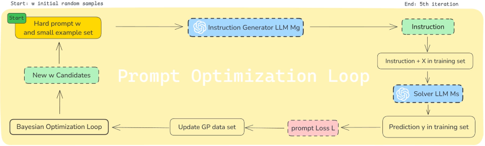
Workflow:

1. Soft prompt $p \in \mathbb{R}^{d \times \tau}$
2. Random projection $A \in \mathbb{R}^{d \times q}$
3. High-dim embedding space로 projection
4. 가장 가까운 token embedding 찾기
5. Hard prompt 복원
6. Instruction generator LLM (Mg) 실행
7. Solver LLM (Ms) 평가
8. BO 업데이트

---

4. 핵심 수식: Penalty-regularized UCB

기존 BO는:

$UCB(p) = \mu(p) + \beta \sigma(p)$

문제:

random projection된 점 Ap[i]가

LLM token embedding과 너무 멀 수 있음 → nonsense instruction 생성

---

4.1 제안된 Penalty 함수 (Eq. 8)

$\pi(p) = \frac{1}{\tau} \sum_{i=1}^{\tau} \min_{e \in E} \|Ap[i] – e\|$

해석:

• 각 projected token이
• 가장 가까운 실제 token embedding과 얼마나 먼지 측정
• 평균 거리

---

4.2 Penalized UCB (Eq. 9)

$p^{(n+1)} = \arg\max_{p \in P} \mu(p) + \beta\sigma(p) – C\pi(p)$

즉:

• exploration/exploitation 유지
• 하지만 embedding space에 가까운 후보만 선호

이게 이 논문의 핵심 기여입니다.

---

5. 왜 중요한가?

기존 방법:

• BO → continuous 탐색
• 이후 rounding
• semantic 붕괴 가능

BOInG:

• 탐색 자체를 embedding manifold 근처로 제한
• 구조적 prior 도입
• LLM-friendly region에서만 탐색

이는 일종의:

Embedding-aware Bayesian Optimization

으로 볼 수 있습니다.

---

6. 실험 결과 (Sec. 4)

6개 task에서 평가

Task	BOInG	InstructZero	Instinct
Synonyms	0.30	0.38	0.30
Common	0.17	0.15	0.21
Letter List	1.00	1.00	1.00
Taxonomy	0.82	0.82	0.85
Word Sorting	0.65	0.64	0.51
Second Word Letter	0.93	0.62	0.10

(표는 p.11 Table 1 기준)

결론:

• 성능은 InstructZero/Instinct와 유사하거나 일부 superior
• compute cost는 압도적으로 낮음

---

7. 계산 자원 비교 (Figure 2, p.3)

Method	GPU	Params	Memory
BOInG	GPT-2 embedding only	38M	~147MB
InstructZero	13B model	26GB
Instinct	13B model	26GB

BOInG는:

• API 기반 black-box 사용
• embedding penalty만 로컬 계산
• white-box LLM full model 불필요

---

8. 이 논문의 본질적 의미

이 논문은 단순한 prompt tuning이 아니라:

“LLM embedding manifold를 고려한 BO”

를 제안한 것.

이는 다음과 연결됩니다:

• Latent BO
• Manifold-constrained optimization
• Trust-region BO
• Adversarial suffix LBO와 유사 개념

---

9. 한계

논문에서 명시한 한계:

1. GPT-2 embedding 사용 → Mg embedding과 mismatch 가능
2. GP surrogate 한계 (high-dim 어려움)
3. categorical handling 문제
4. multi-modal 확장 미검증

---

10. 한 줄 요약

BOInG는 embedding manifold-aware penalty를 도입한 저비용 black-box instruction optimization 방법이다.

---

아래는 **BOInG (Bayesian Optimization for Instruction Generation)**의 방법론을 수식·알고리즘 중심으로 정리한 내용입니다.

---

1. 문제 정식화

두 개의 LLM을 사용합니다.

• $M_g$: Instruction Generator (instruction 생성)
• $M_s$: Solver (downstream task 수행)

목표는 hard prompt $w \in W^\tau (길이 \tau)$를 찾아,

$M_g$가 생성한 instruction을 $M_s$에 넣었을 때 성능을 최대화하는 것:

$\max_{w \in W^\tau} \mathcal{L}\big(w; M_g, M_s, (X,Y)_{\text{small}}, (X,Y)_{\text{eval}}\big)$

논문에서는 (p.8, Eq. (7)) 다음과 같은 정확도 기반 loss를 사용합니다:

$\mathcal{L}(w) = \frac{1}{N} \sum_{i=1}^N \mathbf{1}\{y_i = M_s(M_g(w \oplus (X,Y)) \oplus x_i)\}$

즉:

1. hard prompt $w$ + few-shot examples → $M_g$
2. 생성된 instruction → $M_s$
3. validation 성능 측정

문제점:

$|W|^\tau$의 조합 폭발 (combinatorial explosion)

---

2. Soft Prompt 공간으로 완화

직접 hard prompt를 탐색하지 않고,

$p \in \mathbb{R}^{d \times \tau}$

의 low-dimensional soft prompt 공간에서 BO를 수행합니다.

• $d \ll q$
• $q$: LLM embedding dimension

---

3. Random Projection

soft prompt $p$를 LLM embedding 공간으로 매핑:

$A \in \mathbb{R}^{d \times q}$

$z_i = A p[i]$

• $z_i \in \mathbb{R}^q$
• embedding space $\Omega$

Random projection은 거리 보존 성질을 가짐 (Johnson–Lindenstrauss)

---

4. Hard Prompt 복원

LLM token embedding 집합:

$E = \{e_j\}_{j=1}^{|W|}$

각 projected vector $z_i$에 대해:

$j_i^* = \arg\min_j \| z_i – e_j \|$

$w_i = \text{decode}(e_{j_i^*})$

이렇게 soft prompt → hard prompt 변환.

---

5. 핵심 문제: Projection Drift

문제는:

• $z_i$가 embedding manifold에서 멀 수 있음
• 가장 가까운 token도 여전히 semantic incoherence 가능
• 이상한 instruction 생성

---

6. 제안: Penalty 함수 도입 (Eq. 8)

$\pi(p) = \frac{1}{\tau} \sum_{i=1}^{\tau} \min_{e \in E} \| A p[i] – e \|$

해석:

• projected embedding이 실제 token embedding과 얼마나 떨어져 있는지
• 평균 거리

이 값이 클수록 “비현실적인 soft prompt”

---

7. Penalized UCB

GP surrogate:

$\mu(p), \quad \sigma(p)$

기존 UCB:

$\mu(p) + \beta \sigma(p)$

BOInG의 핵심 수정:

$\text{UCB}_\text{pen}(p) = \mu(p) + \beta \sigma(p) – C \pi(p)$

• $\beta$: exploration–exploitation tradeoff
• C: manifold regularization strength

---

8. Bayesian Optimization Loop

Step 1: 초기화

• Sobol sampling으로 $p^{(1)},…,p^{(n)}$ 생성
• 각각 hard prompt로 변환
• instruction 생성
• 성능 평가

---

Step 2: GP 학습

$\{(p^{(i)}, \mathcal{L}^{(i)})\}$

GP posterior 계산:

$\mu(p) = k(p,P) (K+\lambda^2 I)^{-1} L$

$\sigma^2(p) = k(p,p) – k(p,P)(K+\lambda^2 I)^{-1}k(P,p)$

---

Step 3: Penalized UCB 최적화

$p^{(n+1)} = \arg\max_p \mu(p) + \beta\sigma(p) – C\pi(p)$

이때 동시에 nearest token index 계산.

---

Step 4: Evaluation

• $p^{(n+1)}$ → hard prompt
• instruction 생성
• validation score 계산
• GP 업데이트

---

9. 알고리즘 구조 (Algorithm 2)

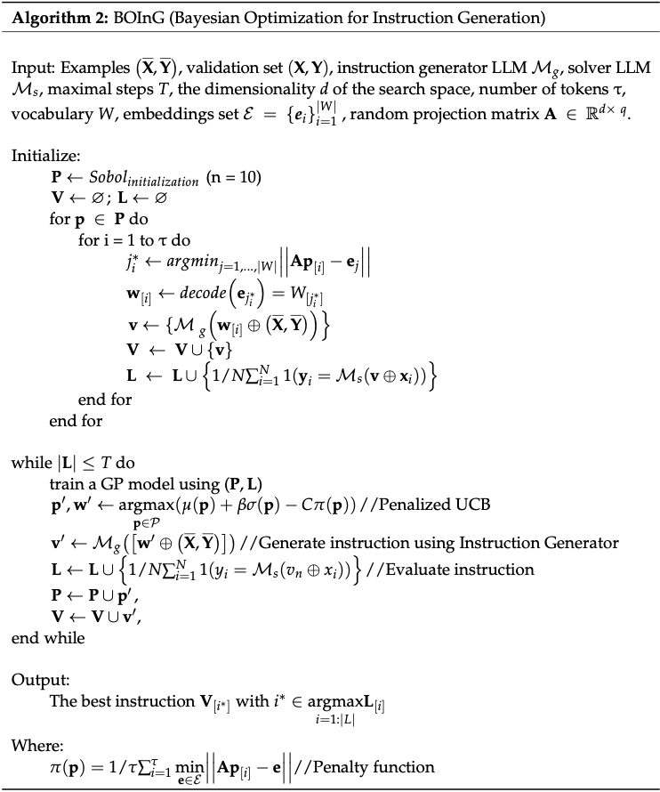
요약:

Initialize P via Sobol
Evaluate initial prompts

while budget not exhausted:
    Fit GP
    p' = argmax (μ + βσ - Cπ)
    Convert to hard prompt
    Generate instruction
    Evaluate score
    Update dataset
return best instruction

---

10. 계산 설정 (실험 세팅)

• τ = 5 tokens
• d = 10
• β = 1
• C = 1
• random projection A ∼ Uniform(-1,1)
• 25 candidates per iteration

---

11. 방법론의 본질

BOInG는 단순히 BO를 쓴 것이 아니라:

Embedding manifold-aware Bayesian Optimization

으로 해석할 수 있습니다.

이는 다음과 유사합니다:

• Trust-region BO
• Manifold-constrained BO
• Latent Bayesian Optimization
• Adversarial suffix LBO (유사 구조)

---

12. 이 접근의 구조적 의미

BOInG는 다음 구조를 갖습니다:

Low-dim search space (P)
        ↓ random projection
High-dim embedding space (Ω)
        ↓ nearest neighbor
Discrete token space (W)

그리고 penalty는

Ω에서의 manifold distance regularization 입니다.

---

다음은 **BOInG (Bayesian Optimization for Instruction Generation)**의 실험 설정과 결과를 구조적으로 정리한 내용입니다.

---

1. 실험 설정

1.1 평가 지표 (Sec. 4.1)

태스크 특성에 따라 네 가지 metric을 사용:

Metric	설명	적용 태스크
Exact Match (EM)	완전 일치 시 1, 아니면 0	Letter List, Second Word Letter
Exact Set (ES)	예측 집합이 정답 집합과 정확히 일치	Taxonomy
Contain	예측이 정답 집합에 포함되면 1	Word Sorting, Synonyms
F1	단어 단위 precision/recall 기반	Common

---

1.2 사용 태스크 (Sec. 4.2)

총 6개 태스크 (InstructZero 논문에서 일부 선택)

Easy

1. Letter List
2. Word Sorting

Challenging

3. Taxonomy
4. Synonyms
5. Second Word Letter
6. Common

---

1.3 하이퍼파라미터

• Soft prompt 길이 $\tau$ = 5
• Latent dimension d = 10
• Random projection $A \sim \mathcal{U}(-1,1)$
• β = 1
• C = 1 (penalty weight)
• 초기 Sobol 샘플 10개
• iteration당 25개 후보 탐색
• LLM: GPT-3.5 Turbo

---

2. 정량 결과 (Table 1)

Task	Difficulty	BOInG	APE	Instinct	InstructZero
Synonyms	Challenging	0.30	0.36	0.30	0.38
Common	Challenging	0.17	0.07	0.21	0.15
Letter List	Easy	1.00	1.00	1.00	1.00
Taxonomy	Challenging	0.82	0.35	0.85	0.82
Word Sorting	Easy	0.65	0.33	0.51	0.64
Second Word Letter	Challenging	0.93	0.75	0.10	0.62

(출처: Table 1, p.11  )

---

3. 결과 해석

3.1 전반적 성능

• InstructZero/Instinct와 거의 동등
• 일부 태스크에서 outperform

특히:

• Second Word Letter: BOInG 0.93 (Instinct 0.10 대비 압도적 우위)
• Word Sorting: BOInG 0.65 (APE 대비 큰 개선)
• Taxonomy: InstructZero와 동일 (0.82)

---

3.2 Easy vs Challenging

Easy Tasks

• 모든 방법이 Letter List에서 1.00
• Word Sorting에서는 BOInG가 Instinct/APE보다 우수

Challenging Tasks

• Common, Synonyms는 여전히 낮은 점수 (본질적으로 어려움)
• Second Word Letter는 BOInG가 크게 우수

→ penalty가 syntactic precision task에서 효과적일 가능성

---

4. 계산 비용 비교 (Figure 2, p.3)

Method	Parameters	Memory	GPU
BOInG	38.6M	~147MB	NVIDIA T4
InstructZero	13B	26GB	A6000
Instinct	13B	26GB	A100

핵심:

• BOInG는 GPT-2 embedding만 로컬 사용
• instruction/solver는 API 호출
• white-box LLM 불필요

---

5. Instruction 진화 예시 (Table 2, p.12)

Synonyms 태스크 예시:

Iteration	Hard Prompt	Generated Instruction	Score
Init	waalf addingolatedprom	Provide synonymous words for each input.	0.40
1	waalf addedolated leng	Provide alternative words for each given input.	0.40
2	ceryalfPOST withdrawnitia	Provide synonyms for the given words.	0.45
3	ceryge Sleepaos safegu	Provide synonymous terms for the given words.	0.55

관찰:

• hard prompt는 거의 랜덤 문자열
• instruction은 점점 명확하고 구체적
• score 점진적 상승

→ BO가 실제로 instruction quality를 개선함을 시사

---

6. 저자들의 결론 (Sec. 5)

• 성능은 SOTA와 동등 수준
• 계산 비용은 현저히 낮음
• black-box LLM만으로 동작 가능

---

7. 비판적 분석

7.1 강점

• low compute
• closed-source LLM 활용 가능
• embedding manifold regularization 효과 입증

7.2 한계

• GPT-2 embedding 사용 → mismatch 가능
• 6개 태스크만 평가 (24개 전체 아님)
• 통계적 유의성 검정 없음
• 반복 실험 variance 미보고

---

8. 연구 관점에서 중요한 포인트

이 결과는 다음을 시사:

1. Embedding-aware constraint는 실제로 도움이 됨
2. Hard rounding BO보다 안정적
3. Latent BO가 instruction engineering에 실용적

---

BOInG에서 사용하는 random projection이 왜 “거리 보존”을 한다고 말할 수 있는지,

그 이론적 근거가 되는 Johnson–Lindenstrauss (JL) Lemma를 수학적으로 정리해 보겠습니다.

---

1. 문제 상황

고차원 공간 $\mathbb{R}^q$에 있는 점들:

$x_1, x_2, \dots, x_n \in \mathbb{R}^q$

이를 더 낮은 차원 $\mathbb{R}^d ( d \ll q )$로 투영하고 싶습니다.

요구사항:

모든 점 쌍의 유클리드 거리가 거의 보존되기를 원함

즉,

$\|x_i – x_j\| \approx \|f(x_i) – f(x_j)\|$

---

2. Johnson–Lindenstrauss Lemma (정식)

임의의 $0 < \varepsilon < 1$에 대해,

점 개수 n이 주어지면,

$d = O\left(\frac{\log n}{\varepsilon^2}\right)$

차원만 확보하면,

임의의 점 집합 $\{x_1, …, x_n\} \subset \mathbb{R}^q$에 대해

다음이 성립하는 선형 사상 $f: \mathbb{R}^q \to \mathbb{R}^d$가 존재합니다:

$(1 – \varepsilon)\|x_i – x_j\|^2 \le \|f(x_i) – f(x_j)\|^2 \le (1 + \varepsilon)\|x_i – x_j\|^2$

즉,

모든 쌍의 거리 왜곡이 $\varepsilon$ 이하

---

3. Random Projection이 왜 이 조건을 만족하는가?

JL lemma의 핵심은:

“랜덤 가우시안 행렬로 투영하면 높은 확률로 거리 보존”

투영:

$f(x) = \frac{1}{\sqrt{d}} A x$

여기서

$A_{ij} \sim \mathcal{N}(0,1)$

또는

$A_{ij} \sim \text{Uniform}(-1,1)$

---

3.1 직관

고차원 벡터의 길이:

$\|x\|^2 = \sum_{k=1}^q x_k^2$

랜덤 선형 조합:

$(Ax)_i = \sum_{k=1}^q A_{ik} x_k$

각 좌표는:

• 평균 0
• 분산 $\|x\|^2$

즉,

$\mathbb{E}[\|Ax\|^2] = d \|x\|^2$

정규화하면:

$\mathbb{E}\left[\left\|\frac{1}{\sqrt{d}}Ax\right\|^2\right] = \|x\|^2$

→ 기대값에서 정확히 보존

---

3.2 왜 높은 확률로 유지되는가?

이는 concentration of measure 현상 때문입니다.

고차원에서:

• 서로 다른 방향의 랜덤 투영은 거의 직교
• 분산이 평균 주변에 집중

Chernoff bound를 사용하면:

$P\left( \left| \|f(x)\|^2 – \|x\|^2 \right| > \varepsilon \|x\|^2 \right) \le 2\exp(-c \varepsilon^2 d)$

따라서:

$d = O(\frac{\log n}{\varepsilon^2})$

이면 모든 점쌍에 대해 보존됨.

---

4. BOInG에서의 의미

BOInG는:

$p \in \mathbb{R}^{d \times \tau}$

를

$Ap \in \mathbb{R}^{q \times \tau}$

로 투영합니다.

JL lemma가 의미하는 것:

• low-dimensional 공간에서의 거리 구조가
• high-dimensional embedding 공간에서도 거의 유지됨

즉,

$\|p_i – p_j\| \approx \|Ap_i – Ap_j\|$

---

5. 왜 이것이 중요한가?

BO는 surrogate model에서 kernel 기반 거리 계산을 합니다:

$k(p_i, p_j) = \exp(-\|p_i – p_j\|^2)$

random projection이 거리 보존하면:

• kernel 구조가 왜곡되지 않음
• low-dim space에서 탐색해도
• high-dim embedding geometry를 유지

---

6. 직관적 이해

고차원 공간에서는:

• 대부분의 벡터가 거의 직교
• 랜덤 방향 투영해도 전체 구조가 크게 붕괴되지 않음

따라서:

고차원 manifold의 전역 구조를 비교적 작은 차원으로 압축 가능

---

7. 한계

JL lemma는:

• 유한한 점 집합에 대해 보장
• 연속 공간 전체에 대해 보장하지 않음
• 점 수 n 증가 시 필요한 d 증가

BOInG에서는:

• 실제 탐색 점 수가 제한적
• 따라서 JL 조건 만족 가능

---

8. LLM 맥락에서 중요한 해석

Embedding 공간은:

• 의미적 거리 구조를 담고 있음

Random projection이 거리 보존하면:

의미 구조의 상대적 관계가 유지될 가능성

그러나:

• semantic manifold는 선형 구조가 아닐 수 있음
• 따라서 완전한 보존은 아님

그래서 BOInG는 penalty term을 추가함.

---

9. 요약

Johnson–Lindenstrauss lemma는 다음을 보장합니다:

랜덤 선형 투영은 $O(\log n / \varepsilon^2)$ 차원만 있어도 점 집합의 거리 구조를 거의 보존한다.

BOInG에서는 이를 활용해:

• low-dim BO 수행
• high-dim embedding space와의 일관성 유지

---

이번에는 BOInG에서 acquisition function을 어떻게 실제로 최적화하는지를 수식–알고리즘–기하학적 관점까지 상세히 정리하겠습니다.

---

1. 최적화 대상: Penalized UCB

BOInG의 acquisition은 다음입니다:

$\mathcal{A}(p) = \mu(p) + \beta \sigma(p) – C \pi(p)$

여기서

• $\mu(p)$: GP posterior mean
• $\sigma(p)$: GP posterior std
• $\pi(p)$: embedding manifold penalty
• $\beta$: exploration 계수
• C: regularization 강도

우리가 실제로 푸는 문제는:

$p^{(n+1)} = \arg\max_{p \in P} \mathcal{A}(p)$

---

2. 왜 이 최적화가 어려운가?

2.1 비선형 + 비미분 가능 구조

$\pi(p) = \frac{1}{\tau} \sum_{i=1}^{\tau} \min_{e \in E} \| A p[i] – e \|$

문제점:

• min 연산 → non-smooth
• nearest-neighbor → piecewise function
• high-dimensional embedding space

따라서:

gradient-based continuous optimizer는 부적합

---

3. BOInG의 실제 acquisition 최적화 방법

논문에서는 다음을 사용합니다:

SampleReducingMCAcquisitionFunction

(진화적/샘플링 기반 탐색)

즉, gradient descent가 아니라:

Population-based search

---

4. 최적화 절차 (구체적)

Step 1: 후보군 샘플링

low-dimensional space $P \subset \mathbb{R}^{d\tau}$에서

• Sobol sequence 초기화
• 이후 iteration마다 25개 후보 샘플 생성

---

Step 2: 각 후보에 대해 계산

각 p에 대해:

① GP posterior 계산

$\mu(p), \quad \sigma(p)$

이는 closed-form:

$\mu(p) = k(p,P)(K+\lambda^2I)^{-1}L$

$\sigma^2(p) = k(p,p) – k(p,P)(K+\lambda^2I)^{-1}k(P,p)$

---

② Penalty 계산

각 token position i:

$z_i = A p[i]$

$\pi(p) = \frac{1}{\tau} \sum_i \min_j \|z_i – e_j\|$

이때:

• 모든 token embedding과 거리 계산
• GPU로 병렬 처리

---

③ Penalized UCB 계산

$\mathcal{A}(p) = \mu(p) + \beta\sigma(p) – C\pi(p)$

---

Step 3: Top-K 선택

• 25개 중 가장 높은 acquisition 값 선택
• 해당 p가 다음 iteration에 사용

---

5. 왜 샘플링 기반인가?

이유 1: penalty가 non-smooth

nearest-neighbor 때문에:

• gradient 불연속
• region마다 다른 active token

이유 2: 차원은 낮음

• d = 10
• τ = 5
• 총 차원 = 50

→ 50차원 정도면 sampling 기반 충분히 가능

---

6. 기하학적 해석

BOInG acquisition은 다음을 동시에 수행:

$\underbrace{\mu(p)}_{\text{exploit}} + \underbrace{\beta\sigma(p)}_{\text{explore}} – \underbrace{C\pi(p)}_{\text{stay on manifold}}$

이는 다음과 동일:

GP 탐색 + embedding manifold trust-region

penalty가 없으면:

• projected point가 embedding convex hull 밖으로 튀어감
• rounding 시 incoherent token 발생

penalty가 있으면:

• 실제 token embedding cluster 근처에서만 탐색

---

7. 최적화 관점에서 보면

이것은 사실:

$\max_p \text{UCB}(p) \quad \text{s.t. } Ap[i] \in \text{neighborhood of } E$

를 $\text{soft constraint}$ 형태로 바꾼 것.

즉: constrained Bayesian optimization의 Lagrangian 형태

---

8. 시간 복잡도 분석

각 acquisition 계산 비용:

GP 계산:

$O(n^2)$

(데이터 포인트 수 n은 매우 작음, 수십 개)

penalty 계산:

$O(\tau |W|)$

• |W| ≈ 50k (GPT-2)
• τ = 5
• GPU 병렬 가능

실제 병목은 penalty 부분.

---

9. 수학적으로 보면

penalty는 사실:

$\pi(p) = \text{dist}(Ap, \mathcal{M})$

여기서 $\mathcal{M}$은

token embedding manifold

따라서 acquisition은:

$\text{UCB}(p) – C \cdot \text{dist}(Ap, \mathcal{M})$

이는

Manifold-Regularized Bayesian Optimization

---

10. 이 구조의 약점

1. nearest-neighbor는 hard assignment
2. embedding mismatch 문제 (GPT-2 vs GPT-3.5)
3. penalty weight C tuning 필요
4. sampling search는 local optimum 위험

---

11. 핵심 요약

BOInG의 acquisition 최적화는:

• Penalized UCB
• Non-smooth manifold constraint
• Sampling-based evolutionary search
• Low-dimensional latent BO

즉,

Constrained, Manifold-aware, Black-box Bayesian Optimization

---