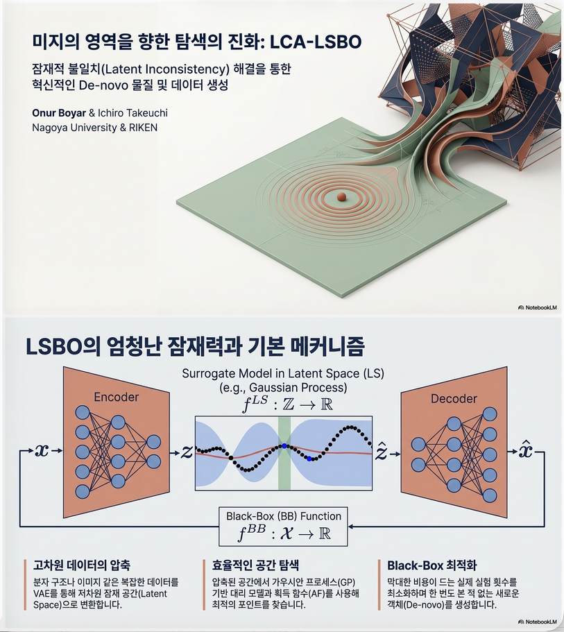
---

1. 연구 배경: Latent Space Bayesian Optimization (LSBO)

1.1 문제: 고차원/구조 데이터 최적화

많은 과학 문제는 다음 형태의 Black-box optimization이다.

$\max_{x \in X} f_{BB}(x)$

예:

• 화학 분자 → docking score
• 이미지 → classifier score
• 단백질 → binding affinity

문제는:

• x 가 고차원 구조 데이터
• 평가 비용이 매우 큼 (실험, 시뮬레이션)

그래서 사용하는 방법이 Bayesian Optimization (BO).

---

1.2 BO의 기본 아이디어

BO는 다음 과정을 반복한다.

(1) surrogate model (보통 Gaussian Process) 학습

$f_{GP}(x)$

(2) acquisition function 사용

$x_{next} = \arg\max AF(x)$

예:

• UCB
• Expected Improvement
• Probability of Improvement

(3) 실제 함수 평가

$y = f_{BB}(x)$

(4) 데이터 업데이트

---

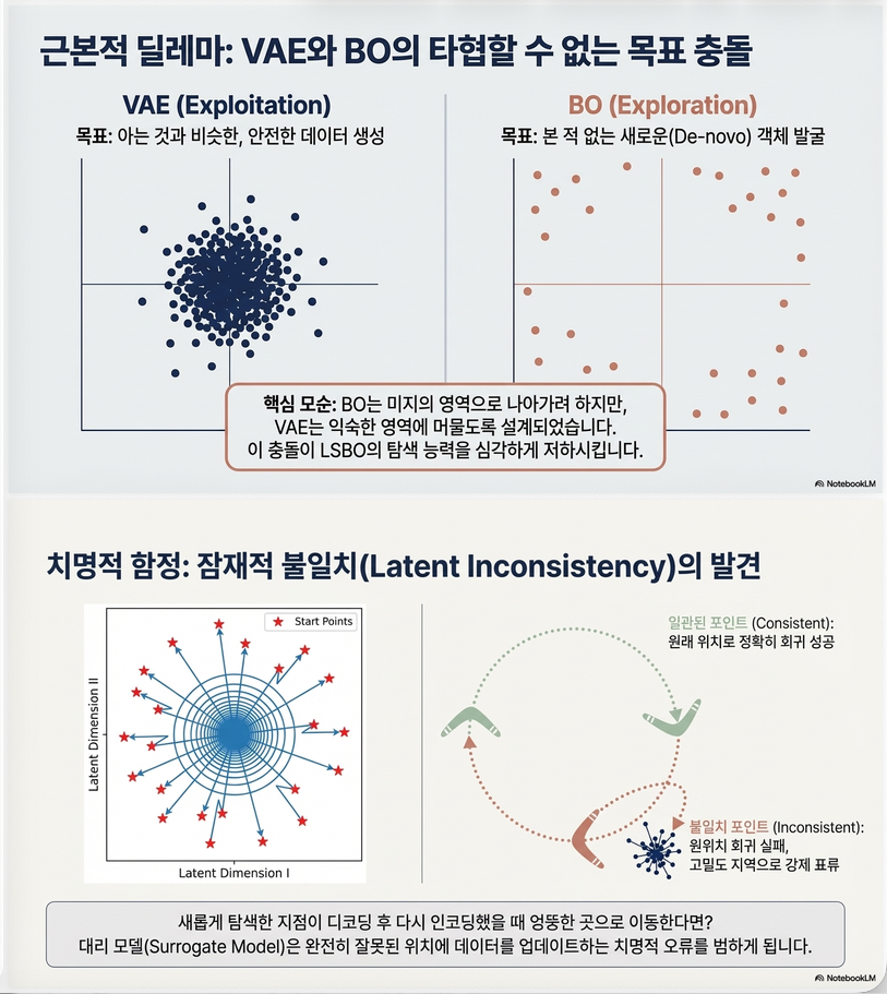
2. LSBO: Latent Space Bayesian Optimization

고차원 문제 해결을 위해 등장한 방법.

핵심 아이디어:

input space X (high dimension)
        ↓
      encoder
        ↓
latent space Z (low dimension)
        ↓
Bayesian Optimization
        ↓
      decoder
        ↓
candidate x

즉

(1) VAE로 latent space 생성

(2) BO는 latent space에서 수행

논문 그림 (p.2) 구조: 

x → encoder → z
z → GP surrogate
z* ← acquisition function
z* → decoder → x*
fBB(x*)

---

3. 기존 LSBO의 핵심 문제

논문의 핵심 contribution은 LSBO의 두 가지 구조적 문제 발견이다.

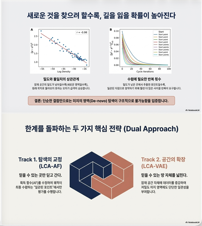
문제 1: VAE–BO objective mismatch

VAE 목적:

training data 근처 샘플 생성

BO 목적:

새로운 영역 탐색

즉

모델	목표
VAE	dense region
BO	sparse region

결과:

• latent space exploration 실패
• off-target generation

---

4. 핵심 개념: Latent Consistency

논문이 새로 정의한 개념.

latent point z 에 대해

decode → encode

하면

$z_1 = f_{enc}(f_{dec}(z))$

latent consistent

$z = z_1$

latent inconsistent

$z \ne z_1$

논문 정의: 

latent variable is consistent if repeated encode–decode cycles converge to the same point.

---

왜 문제가 되는가?

BO는

z → decode → x → fBB(x)

하지만 실제 평가되는 latent point는

$z_1$

즉, BO surrogate는 z에서 학습. 실제 데이터는 z1에서 생성

→ surrogate update mismatch

---

중요한 관찰

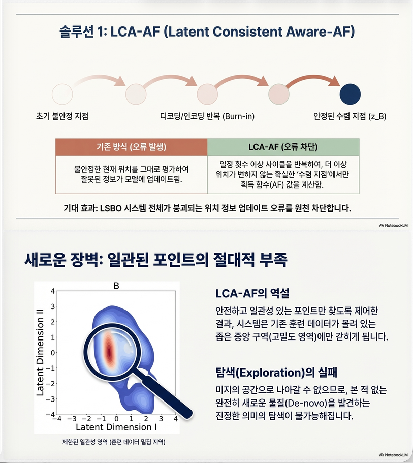
논문 실험 (p.8)

latent density ↓

→ inconsistency ↑

즉

sparse region = inconsistent

하지만 BO는

exploration → sparse region

결과:

BO exploration이 망가짐

---

5. 두 번째 문제: Limited Consistent Points

consistent point는 대부분

latent center

근처에 존재.

즉, exploration 영역에는 consistent point가 거의 없음

결과: LSBO → exploitation only

---

6. 해결 방법

논문은 두 가지 방법 제안.

1. LCA-AF
2. LCA-VAE

그리고 둘을 결합

LCA-LSBO

---

7. Method 1: LCA-AF (Latent Consistency Aware Acquisition Function)

아이디어:

BO가 consistent point만 탐색하도록 한다

방법

latent cycle 수행

z → decode → encode

여러 번 반복

$z_1, z_2, …, z_M$

burn-in 이후

$z_B$를 consistent point로 사용.

Acquisition function 계산:

$\hat f_{LCA-AF}(z) = \frac{1}{M-B} \sum_{j=B}^{M} f_{AF}(z_j)$

실제로는 $f_{AF}(z_B)$ 사용.

---

LCA-AF algorithm

for each BO iteration:

1. GP surrogate 학습
2. z* = argmax LCA-AF
3. x* = decoder(z*)
4. y* = fBB(x*)
5. dataset update
6. VAE retrain

---

8. Method 2: LCA-VAE

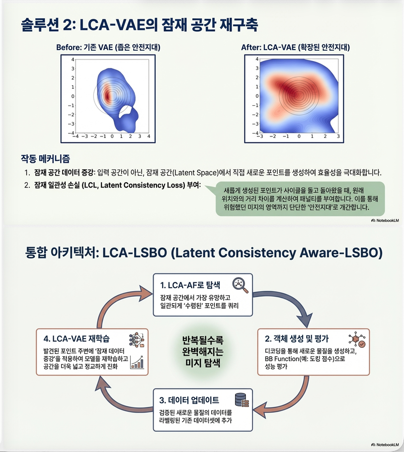
문제: consistent point 수가 너무 적다

해결: latent consistency loss

---

Latent Consistency Loss

$LCL(z) = ||z – z_1||^2$

여기서

$z_1 = enc(dec(z))$

---

새로운 VAE objective

기존: $J_{VAE}$

새 objective:

$J_{LCA-VAE} = J_{VAE} – \gamma E[LCL(z)]$

즉, encode(decode(z)) ≈ z 되도록 latent space 학습.

---

9. Latent Data Augmentation

논문 핵심 아이디어.

기존: data augmentation → input space

논문: data augmentation → latent space

왜?

latent space 장점:

• low dimension
• Gaussian structure
• label-free augmentation

---

Pretraining 단계

reference distribution

$z \sim N(0, \sigma^2 I)$

여기서

$\sigma > 1$

→ sparse region augmentation

---

BO 단계

augmentation 중심

$\mu_{ref} = \arg\max AF$

즉, promising region 주변 latent augmentation

---

10. 최종 알고리즘: LCA-LSBO

전체 흐름

1. LCA-VAE pretrain
2. BO iteration 반복

각 iteration

1 GP 학습
2 z* = argmax LCA-AF
3 x* = decoder(z*)
4 y* = fBB(x*)
5 dataset update
6 latent augmentation
7 LCA-VAE retrain

---

11. 실험

논문은 3개 task 수행.

---

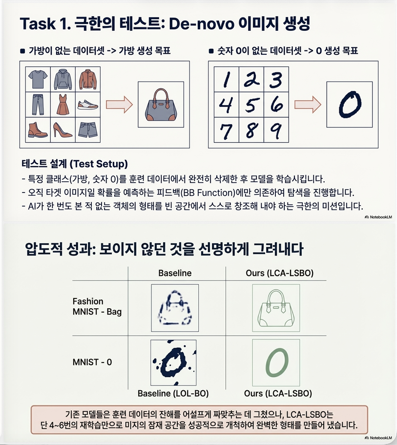
11.1 De-novo Image Generation

두 dataset 사용:

• Fashion-MNIST
• MNIST

실험 설정:

VAE training 시 특정 class 제거

예:

bag 없이 학습
→ bag 생성

또는

digit 0 없이 학습
→ digit 0 생성

---

결과

기존 LSBO: target 생성 실패

LCA-LSBO: few iterations 후 성공

예:

bag generation
4 iteration → bag-like
6 iteration → near-perfect

---

11.2 Chemical Design

dataset: ZINC250K

목표: docking score 최소화

baseline: random 50k molecules

결과

method	best docking
ZINC	-8.80
LCA-LSBO	-9.58

500 iterations 만에 발견. 

---

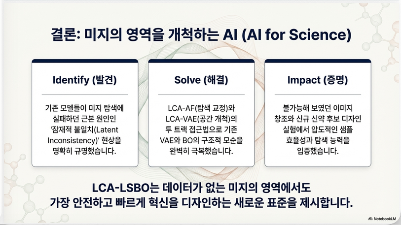
12. 핵심 기여 정리

논문 contribution

(1) Latent Consistency 개념 제안

latent optimization의 핵심 문제 분석.

---

(2) LCA-AF

consistent point 기반 BO.

---

(3) LCA-VAE

latent augmentation + consistency loss.

---

(4) LCA-LSBO

두 방법 결합 → sample-efficient BO.

---

13. 연구적으로 중요한 의미

이 논문은 LSBO 연구에서 중요한 insight 제공.

기존 접근

latent space + BO

이 논문

latent geometry 문제 분석

핵심 메시지

LSBO failure ≠ BO 문제
LSBO failure = latent inconsistency

---

14. LLM 연구와 연결 (중요)

이 논문 아이디어는 최근 LLM 연구와 매우 밀접합니다.

예:

LLM latent BO

• prompt optimization
• jailbreak suffix search
• latent instruction search

대표 논문

• GASP
• LOL-BO
• INSTRUCTZERO
• LBO prompt search

---

특히 중요한 연결

suffix optimization을

token → embedding → BO

로 할 때

exactly 같은 문제 발생

embedding → text → embedding

→ latent inconsistency

---

그래서 이 논문은

LLM latent BO research에서도 매우 중요한 reference

입니다.

---

논문의 **방법론(Methodology)**는 크게 다음 세 가지 구성요소로 이루어집니다.

1. LCA-AF (Latent Consistency-Aware Acquisition Function)
2. LCA-VAE (Latent Consistency-Aware Variational Autoencoder)
3. LCA-LSBO (두 방법을 결합한 최종 LSBO 알고리즘)

각 구성 요소를 문제 정의 → 수식 → 알고리즘 구조 순서로 설명하겠습니다.

---

1. 기본 프레임워크: LSBO

문제 설정:

$\max_{x \in X} f_{BB}(x)$

• $f_{BB}$ : expensive black-box function
• 예: docking score, classifier score 등

하지만 x 가

• 분자
• 이미지
• 구조 데이터

처럼 고차원이기 때문에 BO를 직접 적용하기 어렵습니다.

그래서 사용하는 방법이 Latent Space Bayesian Optimization (LSBO) 입니다.

---

LSBO 구조

입력 공간: $x \in X$

latent 공간: $z \in Z$

VAE 사용: $z = f_{enc}(x)$ , $x = f_{dec}(z)$

BO는 latent space에서 수행됩니다.

BO surrogate: $f_{GP}(z)$

BO iteration:

(1) latent encoding

$z_i = f_{enc}(x_i)$

(2) GP surrogate 학습

$f_{GP}: Z \rightarrow Y$

(3) acquisition optimization

$z^* = \arg\max f_{AF}(z)$

(4) decoding

$x^* = f_{dec}(z^*)$

(5) black-box evaluation

$y^* = f_{BB}(x^*)$

(6) dataset update

---

2. 문제 1: Latent Inconsistency

논문에서 정의한 핵심 개념입니다.

latent point z 에 대해 decode → encode를 수행하면

$z_1 = f_{enc}(f_{dec}(z))$

---

정의

Latent Consistent

$z = z_1$ 또는 $z = z_M$

(encode-decode cycle 반복 후 동일 위치)

---

Latent Inconsistent

$z \ne z_1$

즉 latent point가 decode → encode 후 다른 위치로 이동.

논문 정의: 

A latent point is consistent if repeated encoder-decoder cycles converge to the same point.

---

왜 문제가 되는가

BO는 z 선택

하지만 실제 평가되는 것은

x = decoder(z)

그리고 다시 encoding하면 z1

즉, BO surrogate는 z 기준
실제 데이터는 z1 기준

→ surrogate 학습 오류 발생.

---

3. Method 1: LCA-AF

(Latent Consistency-Aware Acquisition Function)

아이디어: consistent point만 BO에 사용

---

3.1 Latent cycle 계산

latent point z 에 대해 반복:

$z_1 = f_{enc}(f_{dec}(z))$

$z_2 = f_{enc}(f_{dec}(z_1))$

$z_j = f_{enc}(f_{dec}(z_{j-1}))$

논문에서 이를 cycle이라 부릅니다.

---

Algorithm: Latent cycle

Input: z

for j = 1..M
    z_j = enc(dec(z))
    z = z_j

burn-in 이후

$\{z_B, z_{B+1}, …, z_M\}$

를 사용.

---

3.2 Consistent point 판별

consistent point 조건:

$||z_{j+1} – z_j|| \approx 0$

즉 cycle이 수렴.

---

3.3 LCA-AF 계산

기존 acquisition: $f_{AF}(z)$

LCA-AF: $\hat f_{LCA-AF}(z) = \frac{1}{M-B} \sum_{j=B}^{M} f_{AF}(z_j)$

즉, cycle 이후 AF 평균

하지만 실제 구현은 $f_{AF}(z_B)$ 사용.

이렇게 하면 inconsistent point 영향 제거

---

4. Method 2: LCA-VAE

문제:

consistent point 수가 매우 적다

특히, low density region에서 거의 없음.

하지만 BO는 low density region 탐색해야 합니다.

---

4.1 Latent Consistency Loss

latent variable: $\hat z$

cycle 후

$\hat z_1 = enc(dec(\hat z))$

Loss 정의:

$LCL(\hat z) = ||\hat z – \hat z_1||^2$

---

4.2 새로운 VAE objective

기존 VAE objective:

$J_{VAE}(\phi,\theta) = E_{z\sim q_\phi(z|x)} [ \log p_\theta(x|z) – \beta KL(q_\phi(z|x)||p(z)) ]$

---

새 objective:

$J_{LCA-VAE} = J_{VAE} – \gamma E_{\hat z \sim p_{ref}}[LCL(\hat z)]$

여기서

$\gamma$는 hyperparameter.

즉, encode(decode(z)) ≈ z 가 되도록 latent space 학습.

---

5. Latent Data Augmentation

논문의 중요한 아이디어.

기존 augmentation: input space augmentation

문제

• high dimensional
• reconstruction error 증가
• catastrophic forgetting

---

논문 방법: latent space augmentation

---

5.1 Reference distribution

latent augmentation distribution

$p_{ref}(z)$

---

Pretraining 단계

$z \sim N(\mu_{ref}, \sigma_{ref}^2 I)$

보통

$\mu_{ref} = 0$

$\sigma_{ref} > 1$

→ sparse region augmentation.

---

BO 단계

reference center:

$\mu_{ref} = \arg\max \hat f_{LCA-AF}(z)$

즉, BO가 발견한 promising region 주변 augmentation

---

6. 최종 알고리즘: LCA-LSBO

논문의 최종 알고리즘.

---

Algorithm

Step 1: Pretrain LCA-VAE

latent augmentation:

$p_{ref} = N(0, 2I)$

---

Step 2: BO iteration

for j = 1..J

(1) GP surrogate 학습

$f_{GP}(z)$

---

(2) acquisition optimization

$z^* = \arg\max \hat f_{LCA-AF}(z)$

---

(3) decoding

$x^* = f_{dec}(z^*)$

---

(4) black-box evaluation

$y^* = f_{BB}(x^*)$

---

(5) dataset update

---

(6) latent augmentation

$z_i \sim p_{ref}$

---

(7) LCA-VAE retraining

---

7. 전체 구조 요약

기존 LSBO

VAE
  ↓
latent space
  ↓
BO

문제

latent inconsistency
exploration failure

---

논문 방법

LCA-AF
   ↓
consistent point selection

LCA-VAE
   ↓
latent augmentation + consistency loss

최종

LCA-LSBO

---

8. 핵심 아이디어 한 줄 요약

이 논문의 핵심은

LSBO 실패 원인은 BO가 아니라 latent space inconsistency이다.

그래서 consistent latent space + consistent-aware BO를 동시에 설계했습니다.

---

논문의 **실험 결과(Experiments)**는 크게 두 가지 실험 영역으로 구성됩니다.

1. De-novo Image Generation (MNIST / Fashion-MNIST)
2. De-novo Chemical Design (분자 docking score 최적화)

핵심 목적은 다음입니다.

• LSBO가 실제로 새로운 object를 생성할 수 있는지
• sample efficiency가 향상되는지
• 기존 LSBO 방법 대비 성능 향상 여부

아래에서 실험 설정과 결과를 설명하겠습니다.

---

1. De-novo Image Generation 실험

1.1 실험 목적

LSBO의 목표는

$\max f_{BB}(x)$

하지만 논문에서는 이를 interpretable experiment로 설계했습니다.

예:

• VAE가 특정 클래스를 보지 못한 상태
• BO가 그 클래스를 생성하도록 유도

즉, training data에 없는 object 생성을 테스트합니다.

---

1.2 Fashion-MNIST 실험

Fashion-MNIST에는 다음 10개 클래스가 있습니다.

T-shirt
Trouser
Pullover
Dress
Coat
Sandal
Shirt
Sneaker
Ankle boot
Bag

실험 설정:

VAE 학습 시 bag 제거

즉, 9개 클래스만 학습

목표:

BO로 bag 생성

논문 그림 (p.15)에서 설명됩니다. 

---

1.3 MNIST 실험

동일한 구조로 수행됩니다.

예:

digit 0 제거

VAE 학습 데이터

1~9

목표: digit 0 생성

---

1.4 Black-box function

실제 LSBO에서는 expensive function이 필요합니다.

논문에서는 대신 classifier를 사용합니다.

예: bag classifier

score:

$f_{BB}(x) = P(\text{bag}|x)$

즉 BO는 bag 확률을 최대화하도록 탐색합니다.

---

2. 비교 방법 (Baselines)

논문은 9개의 baseline과 비교합니다.

기본 LSBO

• vanilla-VAE
• vanilla-VAE(RT)

(RT = retraining)

---

label-aware VAE

• pred-VAE
• pred-VAE(RT)

---

conditional VAE

• cond-VAE
• cond-VAE(RT)

---

VAE retraining 개선

• weighted-RT
• DML-RT

---

최신 LSBO

• LOL-BO

---

제안 방법

• LCA-AF
• LCA-AF(RT)
• LCA-LSBO

---

3. Retraining 없는 실험 결과

논문 결과 (Table 1, Table 2).

결론: 모든 방법 실패

즉, target class 생성 실패

예:

• bag 생성 실패
• digit 0 생성 실패

논문 설명: 

All methods without retraining completely failed to generate the unseen target instances.

---

왜 실패했는가

VAE 목적:

training data reconstruction

즉, unseen object 생성 불가능

따라서, BO만으로는 insufficient

---

4. Retraining 실험 결과

다음 실험에서는

BO iteration마다 VAE retrain

실험 설정:

BO steps = 10

각 iteration마다 VAE update

---

5. Fashion-MNIST 결과

논문 Figure/Table (p.19). 

주요 결과:

baseline

pred-VAE(RT):

bag 비슷한 shape
하지만 handle 없음

LOL-BO:

일부 클래스만 성공

---

LCA-AF(RT)

성능 향상

bag-like image 생성

---

LCA-LSBO (최고 성능)

결과:

4 iteration → bag-like 등장
6 iteration → 거의 완벽한 bag

즉, 4~6 evaluation만으로 생성 성공.

---

다른 클래스 결과

LCA-LSBO는 다음 클래스 모두 생성 성공.

T-shirt
Trouser
Pullover
Dress
Coat
Sandal
Shirt
Sneaker
Ankle boot
Bag

즉

10 / 10 tasks 성공

---

6. MNIST 결과

MNIST에서도 동일 실험 수행.

baseline 결과:

method	성공 digit
vanilla-VAE(RT)	2
pred-VAE(RT)	3
cond-VAE(RT)	3
LOL-BO	3

---

LCA-AF(RT)

5 / 10 tasks 성공

digits:

0,1,2,3,6,7

---

LCA-LSBO

10 / 10 tasks 성공

즉, 모든 digit 생성

---

7. Chemical Design 실험

논문의 두 번째 핵심 실험입니다.

---

7.1 Dataset

ZINC250K

분자 표현:

SELFIES

(chemical syntax safe representation)

---

7.2 모델

Transformer VAE

Encoder:
8 heads
6 layers

latent dimension:32

---

7.3 목표

단백질

KAT1 protein

binding site:

site18

목표

docking score 최소화

즉, $\min f_{BB}(x)$

---

7.4 Docking 계산

사용 도구

Schrödinger software

절차

molecule → 3D structure
→ docking simulation
→ score

평가 비용

몇 분 ~ 30분

즉, sample efficiency 중요

---

8. Chemical Design 결과

baseline: random 50k molecules

최저 docking score: -8.80

---

LCA-LSBO

500 iteration 후

최저 score: -9.58

논문 Table (p.21). 

Method	Best score
ZINC random	-8.80
LCA-LSBO	-9.58

---

또한

top 3 결과:

Rank	Score
1	-9.58
2	-9.54
3	-9.44

---

Docking score 분포

논문 Figure 5 (p.22) 결과:

LCA-LSBO distribution
↓
더 낮은 score 영역으로 이동

즉, better molecules 발견

---

9. Sample Efficiency

LSBO의 핵심 평가 기준.

결과: 500 evaluations 만으로 50k random search보다 좋은 molecule 발견

즉, 100x 이상 효율적

---

10. 실험 결과 핵심 결론

논문 결과는 다음을 보여줍니다.

---

(1) latent consistency 중요

LCA-AF만 적용해도 성능 향상

---

(2) latent augmentation 중요

LCA-VAE 적용 시, exploration capability 증가

---

(3) 두 방법 결합이 최고

LCA-LSBO가 모든 실험에서 최고 성능.

---

11. 논문 메시지

실험을 통해 입증한 핵심 주장:

LSBO failure ≠ BO problem
LSBO failure = latent inconsistency

따라서, consistent latent space + consistent-aware BO 가 필요합니다.

---